Section 1: Deep-Dive Analysis and Motivation
Surprised by the amount of accidents occuring in New York, our team decided to work with a dataset that could give us more information to help us identify the reasons behind this and see what other developments can be made. Moreover, this information would allow the local community and authorities to understand the scope of the problem, and hopefully would lead to a more informed plan to tackle this issue with better safety policies in place. Our exploratory data analysis (EDA) begins with the goal of deciphering the relevant independent variables as they relate to collisions and injuries/deaths as a result of collisions in New York. Our EDA contains in depth-analysis on the following variables in the merged dataset:
- Borough
- Contributing factor
- Weather; temperature and precipitation (snow, rain, hail)
- Seasons
- Time of day
- Types of death/injuries (pedestrian, car, bicycle)
Section 1.1: Borough
Our first step was to understand which locations in New York have the highest number of accidents. In order to do so, we decided to look into the various boroughs in New York, being the Bronx, Brooklyn, Manhattan, Queens, and Staten Island. We found that Brooklyn observes the highest number of accidents, while Staten Island observes the lowest. This potentially could be because of the narrow roads in Brooklyn and not much population or vehicles in Staten Island. The code for making this observation can be read below. It is important to note that the code below is using the larger dataset instead of the random sample of the original dataset since the random sample values are too small and the plot does not give a distinct answer.
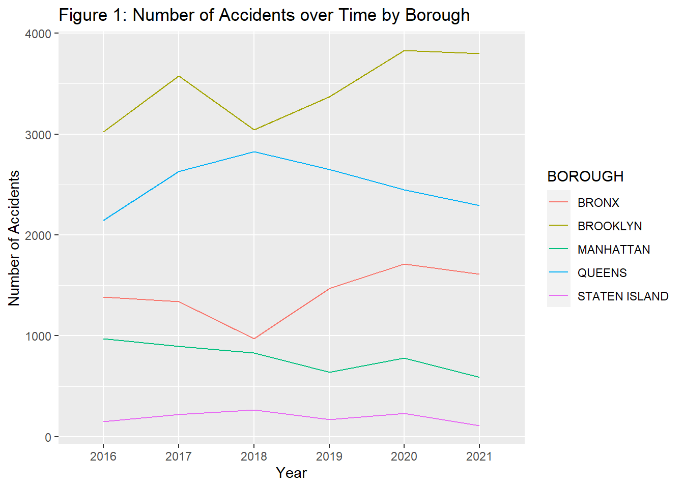
Now that we have a broad understanding of the distribution of accidents across locations, the next question we wanted to answer was what types of accidents these are. For example, are cyclists being hit more than pedestrians and is there a need for better bike law enforcement? These kinds of questions will be answered in the next section.
Section 1.2: Types of death/injuries (pedestrian, motorists, cyclists)
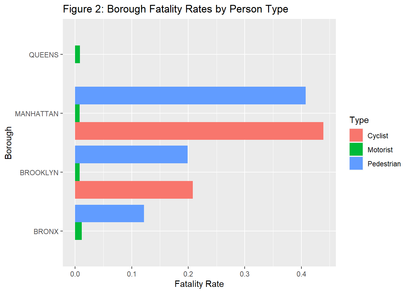
In this section, we will be looking at fatality rates for motorists, cyclists, and pedestrians, respectively. In the code below, we observed that even though overall accidents were much less in Staten Island than in any other borough (Section 1), the highest fatality rates in pedestrians and cyclists are in Staten Island. It is also important to note that in every borough, pedestrians face the highest fatality rates consistently, and motorists face the lowest fatality rates consistently. This tells us that pedestrians are at a much higher risk than other types of people.
We know where they occur and who is impacted by them, but the next question we wanted to answer was why these accidents occur in the first place. This work is motivated by the team’s interpretation of certain reasons being significantly impactful. In the following section, we will be looking at many such contributing factors and make an assessment on which one of these stand out.
Section 1.3: Contributing Factors
In this section, we will be explaining which factors contribute to the likelihood of the occurrence of an accident. The focus in the explanation below is based on the variable that was originally CONTRIBUTING FACTOR VEHICLE 1 from the original dataset, which was eventually renamed to CAUSE. Also, for the purposes of the EDA on the contributing factors, we decided to use the original larger dataset that was too large to include in our github repository.
Our initial dataset contained “contributing factor vehicle code 1” to “contributing factor vehicle code 5.” The variables represent the factor contributing to the collision for a designated vehicle. A high percentage of the contributing factor vehicles 3 to 5 had a significantly high percentage of missing values because there were not many collisions in the dataset that involved more than two vehicles. Additionally, we found that the process for how NYC’s Open Data catalogues the contributing factors for collisions is somewhat inconsistent, and it seems that they attribute the contributing factor for a collision to the variable “contributing factor vehicle 1”, and they didn’t designate a contributing factor to each designated vehicle involved. Most of the two vehicle collision observations would attribute a contributing factor to contributing factor vehicle 1, and for “contributing factor vehicle 2”, it would label the factor as “Unspecified.” Around 83% of the collisions involving two vehicles labelled the contributing factor vehicle 2 as “Unspecified”, and the rest of the collisions would attribute it to all of the other possible contributing factors. Therefore, for the purposes of our analysis we think that “CONTRIBUTING FACTOR VEHICLE 1” should be the only variable relevant to analysis when considering the contributing factors.
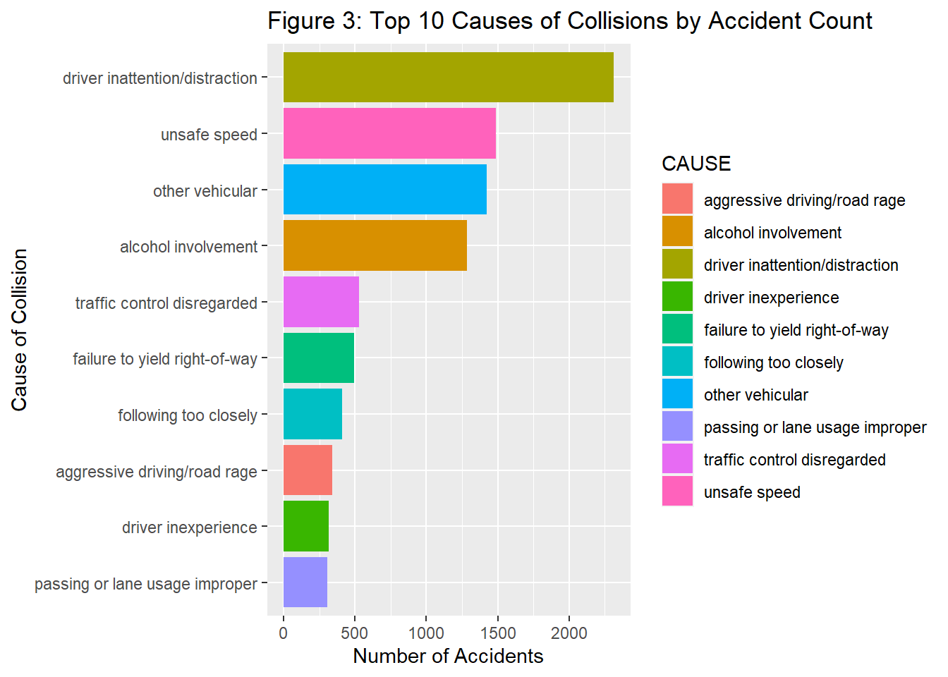
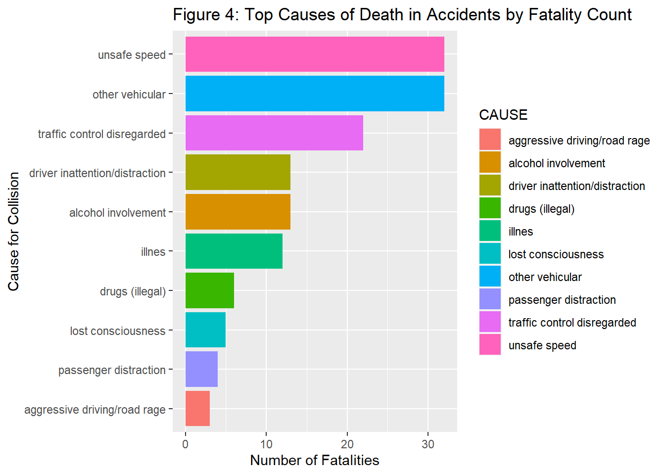
When analyzing the CAUSE variable by accident, we found that ~78% of the total collisions labelled the CAUSE for collision as “unspecified.” For the rest of the EDA, we explored the causes, filtering out the “unspecified” observations because we wanted to understand the causes for collisions at a more descriptive level that could give us more actionable information. When analyzing the causes by accident count filtering “unspecified observations” we found the top cause for collision was “driver inattention/distraction” followed by “unsafe speed”, and “other vehicular”. When analyzing the causes by fatality count, we found that “unsafe speed” was the top cause for collisions leading to a fatality.
| CAUSE | NUMBER_OF_ACCIDENTS | NUMBER_OF_DEATHS |
|---|---|---|
| driver inattention/distraction | 2314 | 13 |
| unsafe speed | 1488 | 32 |
| other vehicular | 1425 | 32 |
| alcohol involvement | 1286 | 13 |
| traffic control disregarded | 528 | 22 |
| failure to yield right-of-way | 493 | 2 |
| following too closely | 412 | 0 |
| aggressive driving/road rage | 343 | 3 |
| driver inexperience | 315 | 0 |
| passing or lane usage improper | 305 | 0 |
| CAUSE | NUMBER_OF_ACCIDENTS | NUMBER_OF_DEATHS |
|---|---|---|
| other vehicular | 1425 | 32 |
| unsafe speed | 1488 | 32 |
| traffic control disregarded | 528 | 22 |
| alcohol involvement | 1286 | 13 |
| driver inattention/distraction | 2314 | 13 |
| illnes | 105 | 12 |
| drugs (illegal) | 92 | 6 |
| lost consciousness | 124 | 5 |
| passenger distraction | 21 | 4 |
| aggressive driving/road rage | 343 | 3 |
Now that there is a good understanding about the relevant variables of the original dataset, we decided to look at a new dataset, namely weather data. This was interesting to think about because our team predicted at least some impact on the number of collisions based on temperature or amount of snow (inches). This is more detailed in section 1.4.
Section 1.4: Weather
Our initial intuition pointed us to analyze how weather affected collisions, as weather has a direct impact on both driving safety and decisions related to travel. We hypothesized forces working in opposite directions. On the one hand, conditions are more dangerous with unfavorable weather conditions, possibly making collisions more likely. However, on the other hand, people are less likely to drive when the weather is poor, reducing traffic volume, and when they do drive, they may drive safer to reduce the chance of a collision.
The following is a graph measuring how the amount of snow, ice pellets, hail, and ice on the ground affects the number of collisions on that day.
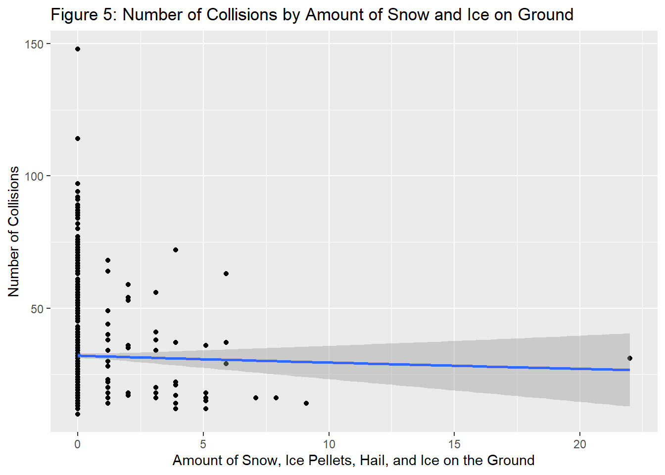 It can be seen that there is almost no correlation between extreme weather and the number of collisions, suggesting that the forces working against each other described above exhibit a relatively equal balancing effect.
We also wanted to examine whether or not extreme weather has an effect on the severity of collisions. To do this, we created a similar graph measuring how the amount of snow, ice pellets, hail, and ice on the ground affects the number of injuries.
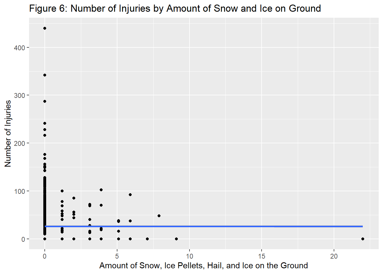 The analysis above again displays relatively little correlation between the variables, and suggests that more extreme weather might actually reduce the severity of collisions, likely due to slower driving in the face of unfavorable conditions.
Finally, we created the same graph on deaths rather than injuries.
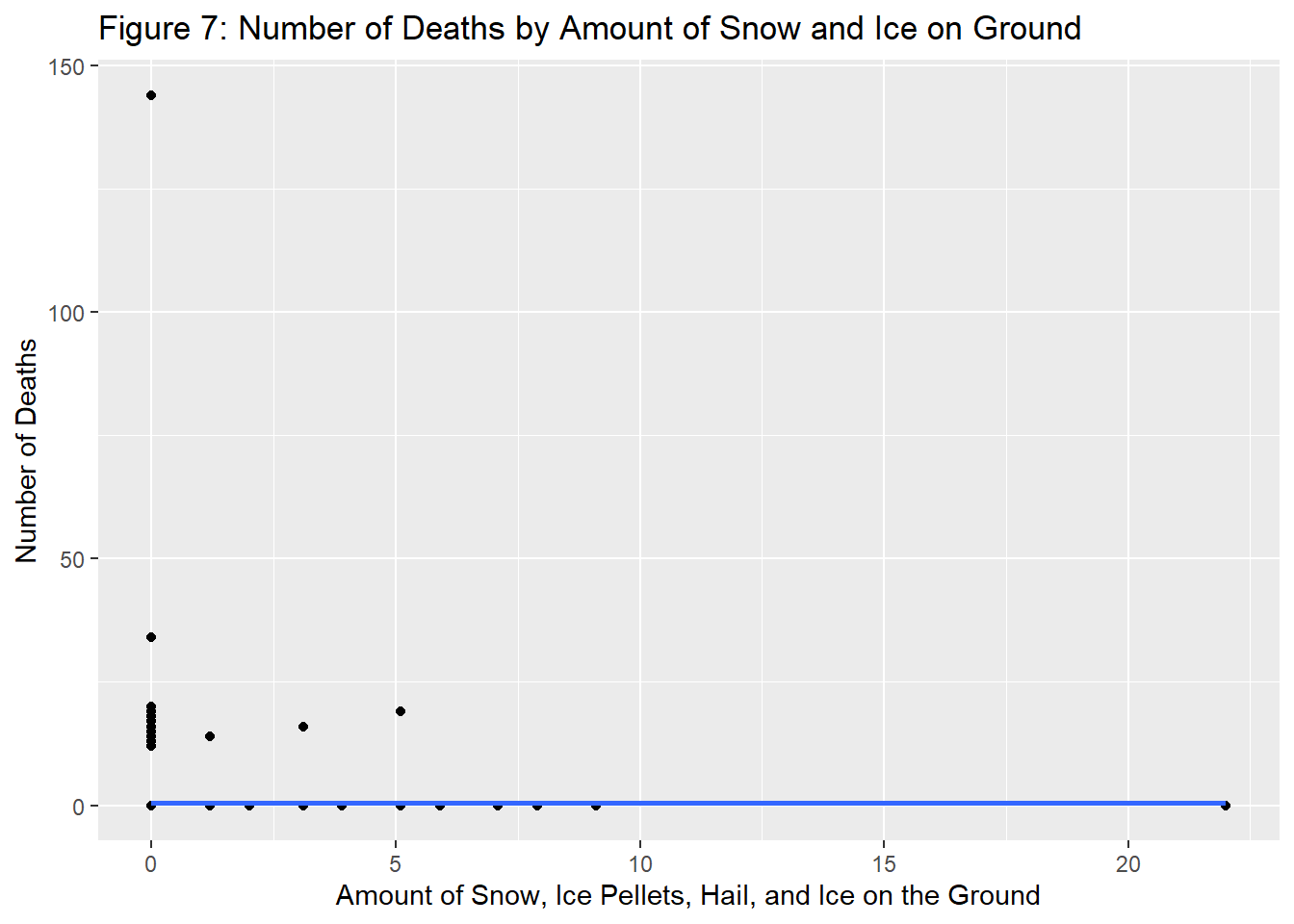 While there is not a ton of correlation, there does appear to be a slight reduction in deaths as a result of more extreme weather. This is more evidence for the fact that while collisions are stable when there is more extreme weather, they are less likely to be severe (though, by a small amount).
This led us to our next variable to measure the effect on collisions: temperature. Below is a graph displaying how the high temperature in New York on a given day affects the number of collisions.
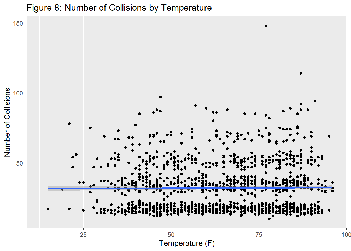 There is only very slight correlation between these two variables between these two variables. However, the same analysis was also conducted with the number of injuries as the y variable rather than the number of collisions.
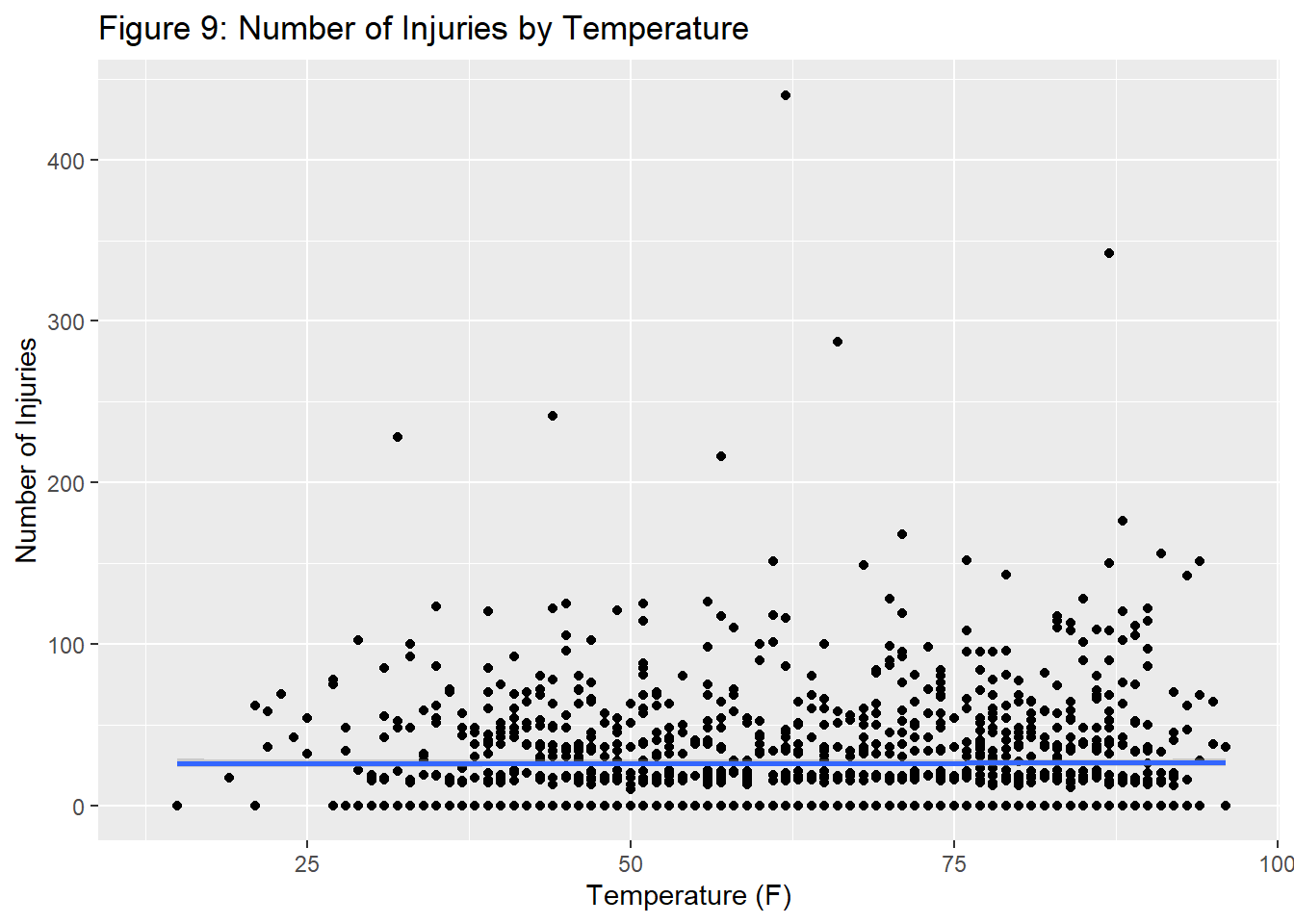 Here, it can be seen that while collisions are stable across temperatures, there is slightly more correlation between the temperature and the number of injuries.
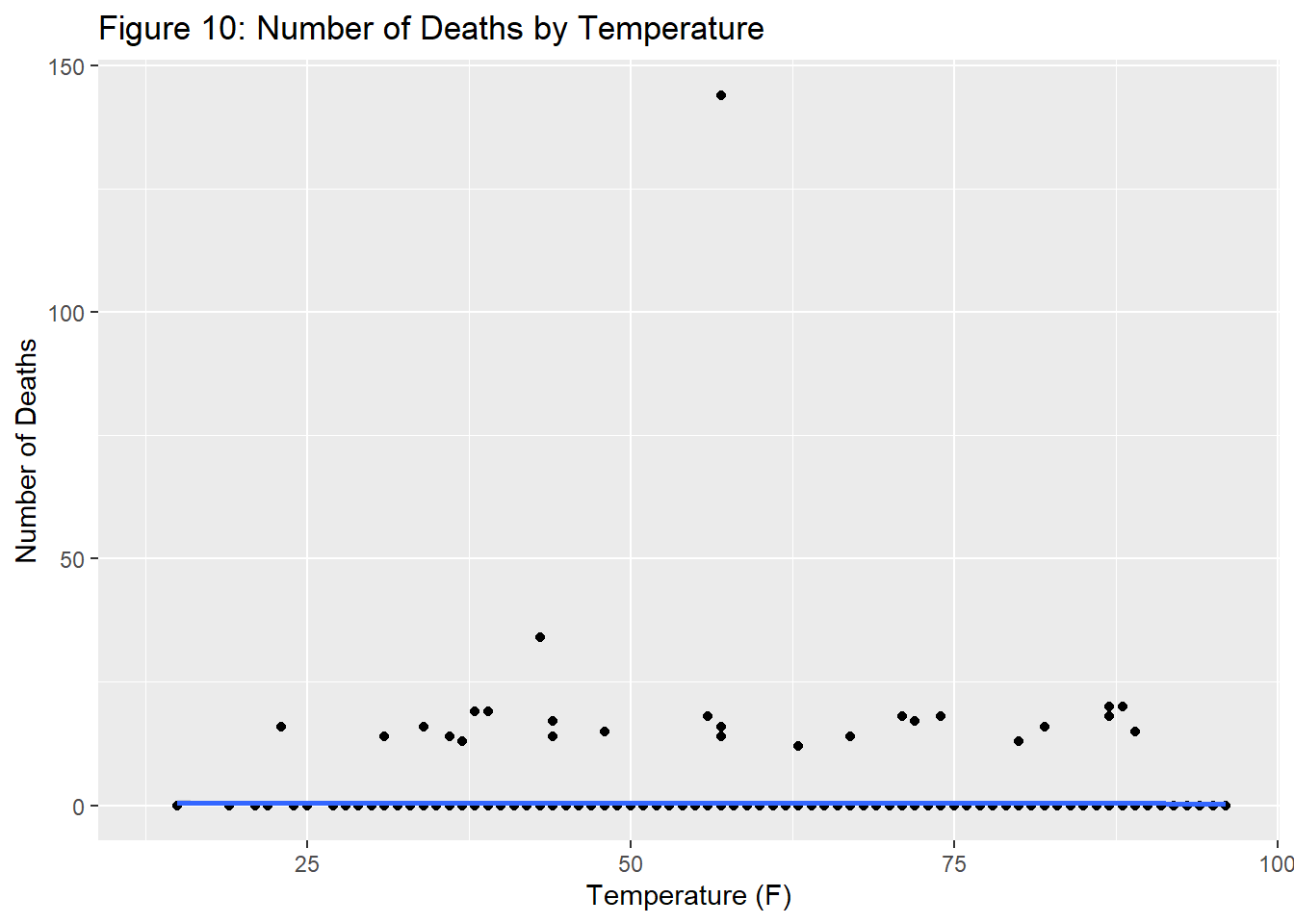
A similar graph run on deaths rather than injuries shows the same trend, though the numbers are far too small to be conclusive.
 The relationship between temperature, the number of collisions and the severity of the accident (which is defined by the number of injuries/deaths) provides the most interesting avenue to explore further within the weather dataset. In order to dive deeper into this relationship, we coded in a seasons variable. The next section focuses on analysis related to the season, showing how the prevalence of types of injuries changes by season.
Section 1.4.1: Seasons
The following table displays the number of injuries by season, splitting up the type of injury (between motorists, cyclists, and pedestrians). These numbers represent totals for the entire five-year span in the dataset.
| SEASON | Pedestrians Injured | Motorists Injured | Cyclists Injured | People Injured |
|---|---|---|---|---|
| Winter | 230 | 8060 | 54 | 8344 |
| Summer | 217 | 8788 | 77 | 9082 |
| Spring | 304 | 6989 | 51 | 7344 |
| Fall | 215 | 8138 | 113 | 8466 |
It is clear that injuries are higher in the summer and fall than the winter and spring. A spike in cyclist injuries when it is warmer is evident, but this cannot fully account for the difference in injuries because the number of motorists injured is also significantly higher in the summer and fall.
As a result of the EDA on weather and seasons, it was clear that there were behavioral differences as a result of these two factors that led to variation in the number of collisions and the severity of the collisions. In order to delve deeper into the analysis, it is imperative to map out the collisions on a New York City map in order to identify clusters and trends with how, where, and when different types of collisions are taking place. Some insights using this method are present in the big picture page.
Section 1.5: Time of Day
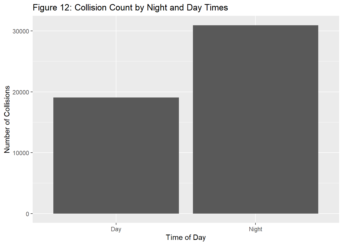
Another variable that we wanted to observe was time of day and how drivers may be more at risk during certain hours. This was motivated by our expectation of two main timings in a given day where there would be a noticeable increase in collisions: evening and morning rush hours since a metropolitan area such as NYC would likely have very busy traffic patterns, and later hours into the night, as we thought there would be more instances of driving under the influence. To verify these assumptions, we created the graph shown below to visualize the distribution of collisions based on hourly data.
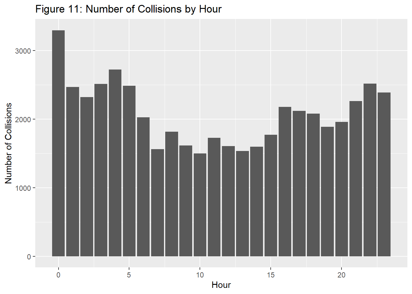 From this graph, the general trend seems to be that collisions are actually lower during mornings (around 10am), and tend to increase over the rest of the afternoon into very early mornings (before 5am). From this trend, it appears that NYC collisions tend to be influenced by the level of visibility and how light or dark it is. With sunrise and sunset times in New York being around 7am and 5pm respectively, sunlight seems to play a significant role in collision volume. Mutating a new variable to reflect these sunrise and sunset, we see the following distribution.
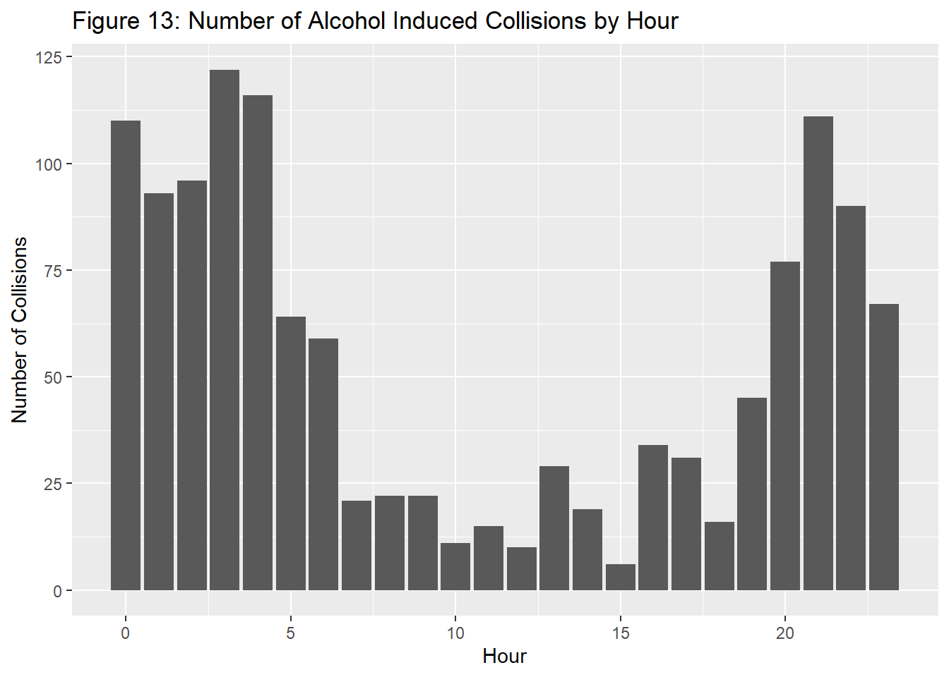
 After isolating for alcohol involvement, the following graph was created.It’s evident that there is a clear trend with driving under the influence of alcohol and time of day. Number of collisions peaks between midnight and 4am for drunk drivers, thus it’s safe to assume this is a time period to avoid as there will likely be a higher concentration of drunk drivers.
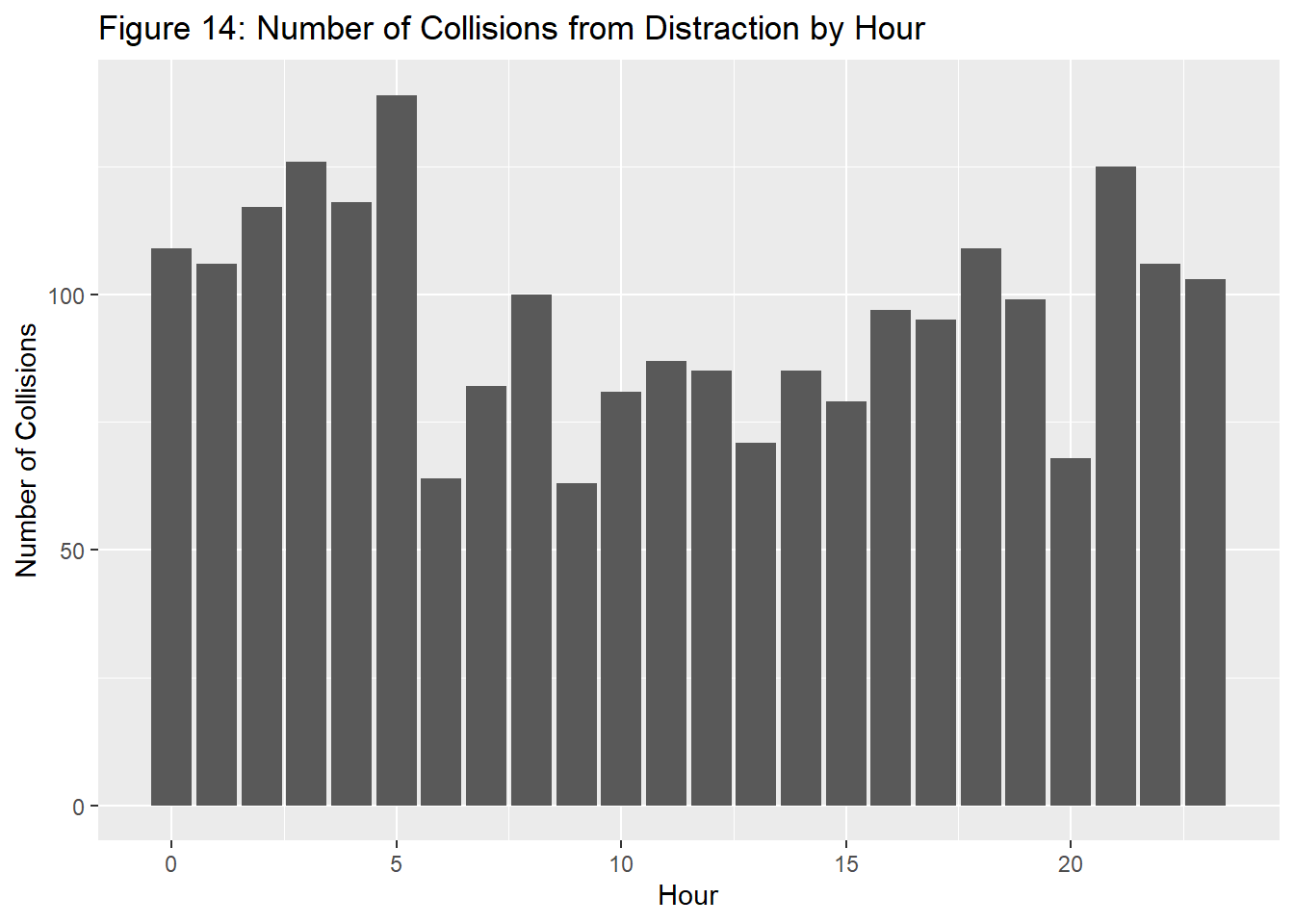
It’s also during this same time that involves the highest amount of distracted drivers, as seen from the graph below. This likely plays into the visibility trends seen prior, as distractions will be intensified without the visual awareness that drivers have during the daytime.
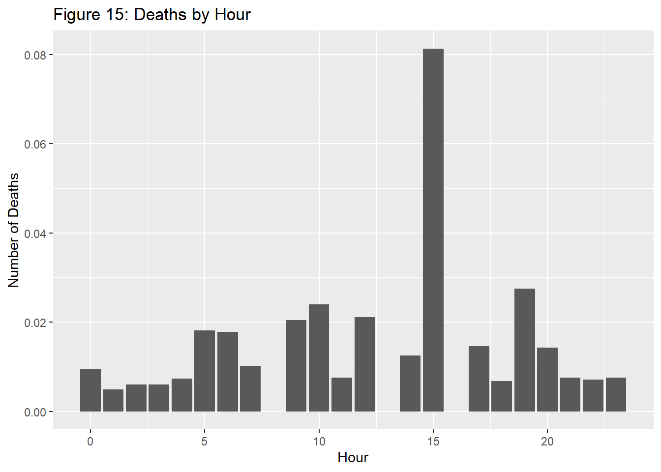
 After understanding the above trends, we wanted to see the impact of these collisions at specific times during the day. Looking at death rates per hour rather than collision count per hour tells a different story from the visual shown below. Though it seems that rush hour didn’t yield any significance in the raw number of collisions, accidents in New York City are more likely to result in death during afternoon and rush hour. As seen in the graph, there was a dramatic increase in hour 15(3 pm). After further research, at this time on October 31st 2017, a tragedy occurred killing 8 people and injuring 12. Since this dataset is based on police reportings, this point was duplicated multiple times, explaining the figure seen here.
Section 2: Modeling and Inferences
We ran numerous linear regressions on weather data, as displayed below.
## Warning in eval(predvars, data, env): NAs introduced by coercion## MODEL INFO:
## Observations: 1282 (545 missing obs. deleted)
## Dependent Variable: NUMBER OF PERSONS INJURED
## Type: OLS linear regression
##
## MODEL FIT:
## F(1,1280) = 0.08, p = 0.78
## R² = 0.00
## Adj. R² = -0.00
##
## Standard errors: OLS
## -------------------------------------------------------------
## Est. S.E. t val. p
## ------------------------------ ------- ------ -------- ------
## (Intercept) 26.17 1.02 25.54 0.00
## as.numeric(`SNOW, ICE -0.29 1.04 -0.28 0.78
## PELLETS, HAIL, ICE ON GROUND
## (IN)`)
## -------------------------------------------------------------## Warning in eval(predvars, data, env): NAs introduced by coercion## MODEL INFO:
## Observations: 1282 (545 missing obs. deleted)
## Dependent Variable: num_collisions
## Type: OLS linear regression
##
## MODEL FIT:
## F(1,1280) = 1.64, p = 0.20
## R² = 0.00
## Adj. R² = 0.00
##
## Standard errors: OLS
## -------------------------------------------------------------
## Est. S.E. t val. p
## ------------------------------ ------- ------ -------- ------
## (Intercept) 32.14 0.50 63.77 0.00
## as.numeric(`SNOW, ICE -0.66 0.51 -1.28 0.20
## PELLETS, HAIL, ICE ON GROUND
## (IN)`)
## -------------------------------------------------------------## MODEL INFO:
## Observations: 1298 (529 missing obs. deleted)
## Dependent Variable: num_collisions
## Type: OLS linear regression
##
## MODEL FIT:
## F(1,1296) = 1.41, p = 0.23
## R² = 0.00
## Adj. R² = 0.00
##
## Standard errors: OLS
## ------------------------------------------------
## Est. S.E. t val. p
## ----------------- ------- ------ -------- ------
## (Intercept) 29.93 1.85 16.17 0.00
## TEMP HIGH 0.03 0.03 1.19 0.23
## ------------------------------------------------## MODEL INFO:
## Observations: 1298 (529 missing obs. deleted)
## Dependent Variable: NUMBER OF PERSONS INJURED
## Type: OLS linear regression
##
## MODEL FIT:
## F(1,1296) = 0.73, p = 0.39
## R² = 0.00
## Adj. R² = -0.00
##
## Standard errors: OLS
## ------------------------------------------------
## Est. S.E. t val. p
## ----------------- ------- ------ -------- ------
## (Intercept) 23.09 3.76 6.15 0.00
## TEMP HIGH 0.05 0.06 0.86 0.39
## ------------------------------------------------## Warning in eval(predvars, data, env): NAs introduced by coercion## MODEL INFO:
## Observations: 1282 (545 missing obs. deleted)
## Dependent Variable: NUMBER OF PERSONS KILLED
## Type: OLS linear regression
##
## MODEL FIT:
## F(1,1280) = 0.22, p = 0.64
## R² = 0.00
## Adj. R² = -0.00
##
## Standard errors: OLS
## ------------------------------------------------------------
## Est. S.E. t val. p
## ------------------------------ ------ ------ -------- ------
## (Intercept) 0.46 0.13 3.42 0.00
## as.numeric(`SNOW, ICE 0.06 0.13 0.47 0.64
## PELLETS, HAIL, ICE ON GROUND
## (IN)`)
## ------------------------------------------------------------## MODEL INFO:
## Observations: 1298 (529 missing obs. deleted)
## Dependent Variable: NUMBER OF PERSONS KILLED
## Type: OLS linear regression
##
## MODEL FIT:
## F(1,1296) = 1.44, p = 0.23
## R² = 0.00
## Adj. R² = 0.00
##
## Standard errors: OLS
## ------------------------------------------------
## Est. S.E. t val. p
## ----------------- ------- ------ -------- ------
## (Intercept) 1.02 0.49 2.10 0.04
## TEMP HIGH -0.01 0.01 -1.20 0.23
## ------------------------------------------------Additionally, we created a logistic regression model to analyze whether any of the specific contributing factors had a significant impact on whether or not a fatality occurred. The independent variable for the model was the categorical variable CAUSE, which represents the contributing factor for the collision, and we created a binary dependent variable, which represented whether or not the collision resulted in death; 0: No Death, 1: Death. There were some causes with positive coefficients like “driver inattention/distraction,” “alcohol involvement,” “passenger distraction,” and “unsafe speed.”The results of the logistic regression yielded high p-values for each of the contributing factors, indicating that there was not any conclusive evidence to suggest any of the contributing factors had a significant effect on whether a fatality occurred. This result could mean that none of the contributing factors are related to whether or not a fatality occurred, or another possible explanation for the results is that our sample size is too small, and there wasn’t enough evidence in the data to conclude that there is a significant relationship between any of the contributing factors and whether a fatality occurs. This is because while there are over a million observations in our data, a very small percentage of those results in death, leading to little variation between causes.
Thus, using all the variables excluding the cause of the collision, we ran our final model on a binary variable determining whether anyone was injured or died during a collision, yielding the logistic regression output shown below. Each factor proved to be significant here as predictors of injury or death. Out of the boroughs, it seems that the Bronx has the highest likelihood of a collision ending in injury or death, with Staten Island holding the lowest likelihood. In addition, with regards to weather, snowy and icy roads are by far the most impactful hazard, with likelihood of injury/death increasing by .51. Rain also seems to have a presence in dangerous collisions, causing injury/death rate to rise by .05. However, contrary to our beliefs, driving at night at a glance seems to be safer than driving during the day. However, from our EDA, the difference in collision volume was extreme, which implies that this coefficient isn’t as reliable as the others and the relationship likely occurs from the high number of night time collisions.
## MODEL INFO:
## Observations: 41602 (8398 missing obs. deleted)
## Dependent Variable: injury_death
## Type: Generalized linear model
##   Family: binomial
##   Link function: logit
##
## MODEL FIT:
## <U+03C7>²(9) = 494.33, p = 0.00
## Pseudo-R² (Cragg-Uhler) = 0.02
## Pseudo-R² (McFadden) = 0.01
## AIC = 55921.30, BIC = 56007.66
##
## Standard errors: MLE
## ---------------------------------------------------------
##                               Est.   S.E.   z val.      p
## -------------------------- ------- ------ -------- ------
## (Intercept)                  -0.21   0.05    -4.26   0.00
## NIGHTNight                   -0.33   0.02   -15.93   0.00
## BOROUGHBROOKLYN              -0.07   0.03    -2.37   0.02
## BOROUGHMANHATTAN             -0.32   0.04    -7.79   0.00
## BOROUGHQUEENS                -0.20   0.03    -6.48   0.00
## BOROUGHSTATEN ISLAND         -0.38   0.07    -5.50   0.00
## TEMP HIGH                     0.00   0.00     3.65   0.00
## RAIN                          0.05   0.02     2.20   0.03
## SNOW                         -0.21   0.05    -4.35   0.00
## SNOWGROUND                    0.57   0.05    11.58   0.00
## ---------------------------------------------------------