Loading and Cleaning:
library(tidyverse)## -- Attaching packages --------------------------------------- tidyverse 1.3.1 --## v ggplot2 3.3.5 v purrr 0.3.4
## v tibble 3.1.4 v dplyr 1.0.7
## v tidyr 1.1.3 v stringr 1.4.0
## v readr 2.0.1 v forcats 0.5.1## -- Conflicts ------------------------------------------ tidyverse_conflicts() --
## x dplyr::filter() masks stats::filter()
## x dplyr::lag() masks stats::lag()library(dplyr)
library(lubridate)##
## Attaching package: 'lubridate'## The following objects are masked from 'package:base':
##
## date, intersect, setdiff, unioncollision <- read_csv(here::here('dataset/NYC Collision Data.csv'))## Rows: 1831755 Columns: 29## -- Column specification --------------------------------------------------------
## Delimiter: ","
## chr (17): CRASH DATE, CRASH TIME, BOROUGH, LOCATION, ON STREET NAME, CROSS S...
## dbl (12): ZIP CODE, LATITUDE, LONGITUDE, NUMBER OF PERSONS INJURED, NUMBER O...##
## i Use `spec()` to retrieve the full column specification for this data.
## i Specify the column types or set `show_col_types = FALSE` to quiet this message.collision['collision_date'] = as.Date(collision$'CRASH DATE', format="%m/%d/%Y")
collision<- collision%>%mutate(., YEAR = year(collision_date))
collision<- collision%>%filter(YEAR>2015 & YEAR<2021)
summary(collision)## CRASH DATE CRASH TIME BOROUGH ZIP CODE
## Length:1016774 Length:1016774 Length:1016774 Min. :10000
## Class :character Class :character Class :character 1st Qu.:10451
## Mode :character Mode :character Mode :character Median :11208
## Mean :10859
## 3rd Qu.:11249
## Max. :11697
## NA's :360780
## LATITUDE LONGITUDE LOCATION ON STREET NAME
## Min. : 0.00 Min. :-201.36 Length:1016774 Length:1016774
## 1st Qu.:40.67 1st Qu.: -73.97 Class :character Class :character
## Median :40.72 Median : -73.92 Mode :character Mode :character
## Mean :40.67 Mean : -73.83
## 3rd Qu.:40.77 3rd Qu.: -73.86
## Max. :43.34 Max. : 0.00
## NA's :92548 NA's :92548
## CROSS STREET NAME OFF STREET NAME NUMBER OF PERSONS INJURED
## Length:1016774 Length:1016774 Min. : 0.0000
## Class :character Class :character 1st Qu.: 0.0000
## Mode :character Mode :character Median : 0.0000
## Mean : 0.2841
## 3rd Qu.: 0.0000
## Max. :31.0000
## NA's :17
## NUMBER OF PERSONS KILLED NUMBER OF PEDESTRIANS INJURED
## Min. :0.000000 Min. : 0.00000
## 1st Qu.:0.000000 1st Qu.: 0.00000
## Median :0.000000 Median : 0.00000
## Mean :0.001224 Mean : 0.04979
## 3rd Qu.:0.000000 3rd Qu.: 0.00000
## Max. :8.000000 Max. :27.00000
## NA's :31
## NUMBER OF PEDESTRIANS KILLED NUMBER OF CYCLIST INJURED
## Min. :0.000000 Min. :0.00000
## 1st Qu.:0.000000 1st Qu.:0.00000
## Median :0.000000 Median :0.00000
## Mean :0.000621 Mean :0.02474
## 3rd Qu.:0.000000 3rd Qu.:0.00000
## Max. :6.000000 Max. :3.00000
##
## NUMBER OF CYCLIST KILLED NUMBER OF MOTORIST INJURED NUMBER OF MOTORIST KILLED
## Min. :0.0000000 Min. : 0.0000 Min. :0.000000
## 1st Qu.:0.0000000 1st Qu.: 0.0000 1st Qu.:0.000000
## Median :0.0000000 Median : 0.0000 Median :0.000000
## Mean :0.0001131 Mean : 0.2094 Mean :0.000488
## 3rd Qu.:0.0000000 3rd Qu.: 0.0000 3rd Qu.:0.000000
## Max. :2.0000000 Max. :31.0000 Max. :4.000000
##
## CONTRIBUTING FACTOR VEHICLE 1 CONTRIBUTING FACTOR VEHICLE 2
## Length:1016774 Length:1016774
## Class :character Class :character
## Mode :character Mode :character
##
##
##
##
## CONTRIBUTING FACTOR VEHICLE 3 CONTRIBUTING FACTOR VEHICLE 4
## Length:1016774 Length:1016774
## Class :character Class :character
## Mode :character Mode :character
##
##
##
##
## CONTRIBUTING FACTOR VEHICLE 5 COLLISION_ID VEHICLE TYPE CODE 1
## Length:1016774 Min. :3363355 Length:1016774
## Class :character 1st Qu.:3618219 Class :character
## Mode :character Median :3872688 Mode :character
## Mean :3872628
## 3rd Qu.:4127036
## Max. :4463721
##
## VEHICLE TYPE CODE 2 VEHICLE TYPE CODE 3 VEHICLE TYPE CODE 4
## Length:1016774 Length:1016774 Length:1016774
## Class :character Class :character Class :character
## Mode :character Mode :character Mode :character
##
##
##
##
## VEHICLE TYPE CODE 5 collision_date YEAR
## Length:1016774 Min. :2016-01-01 Min. :2016
## Class :character 1st Qu.:2017-02-13 1st Qu.:2017
## Mode :character Median :2018-03-22 Median :2018
## Mean :2018-04-02 Mean :2018
## 3rd Qu.:2019-05-05 3rd Qu.:2019
## Max. :2020-12-31 Max. :2020
## collision_use <- collision %>% filter(!is.na(BOROUGH), !is.na('ZIP CODE'), !is.na(LONGITUDE), !is.na(LATITUDE), !is.na(LOCATION))%>% select(-(`ON STREET NAME`:`OFF STREET NAME`)) %>%
rename(DATE = `CRASH DATE`, TIME = `CRASH TIME`, ZIPCODE = `ZIP CODE`, LOCATION = `LOCATION`)
collision_use['collision_date'] = as.Date(collision_use$DATE, format="%m/%d/%Y")
collision_use<- collision_use%>% mutate(., year = year(collision_date))
collision_use$TIME<- as.character(collision_use$TIME)
collision_use$TIME <- as.numeric(unlist(strsplit(collision_use$TIME, ":"))[seq(1, 2 * nrow(collision_use), 2)])
#EDA
collisions_per_day <-collision_use %>%
group_by(collision_date, BOROUGH) %>%
summarise(NUMBER_OF_ACCIDENTS=n(),
NUMBER_OF_DEATHS = sum(`NUMBER OF PERSONS KILLED`),
NUMBER_OF_INJURIES = sum(`NUMBER OF PERSONS INJURED`))%>%
ungroup()## `summarise()` has grouped output by 'collision_date'. You can override using the `.groups` argument.ggplot(data=collisions_per_day, aes(x=collision_date, y=NUMBER_OF_ACCIDENTS))+
geom_line(aes(group=BOROUGH, color=BOROUGH))+ggtitle("Number of Accidents over Time by Borough")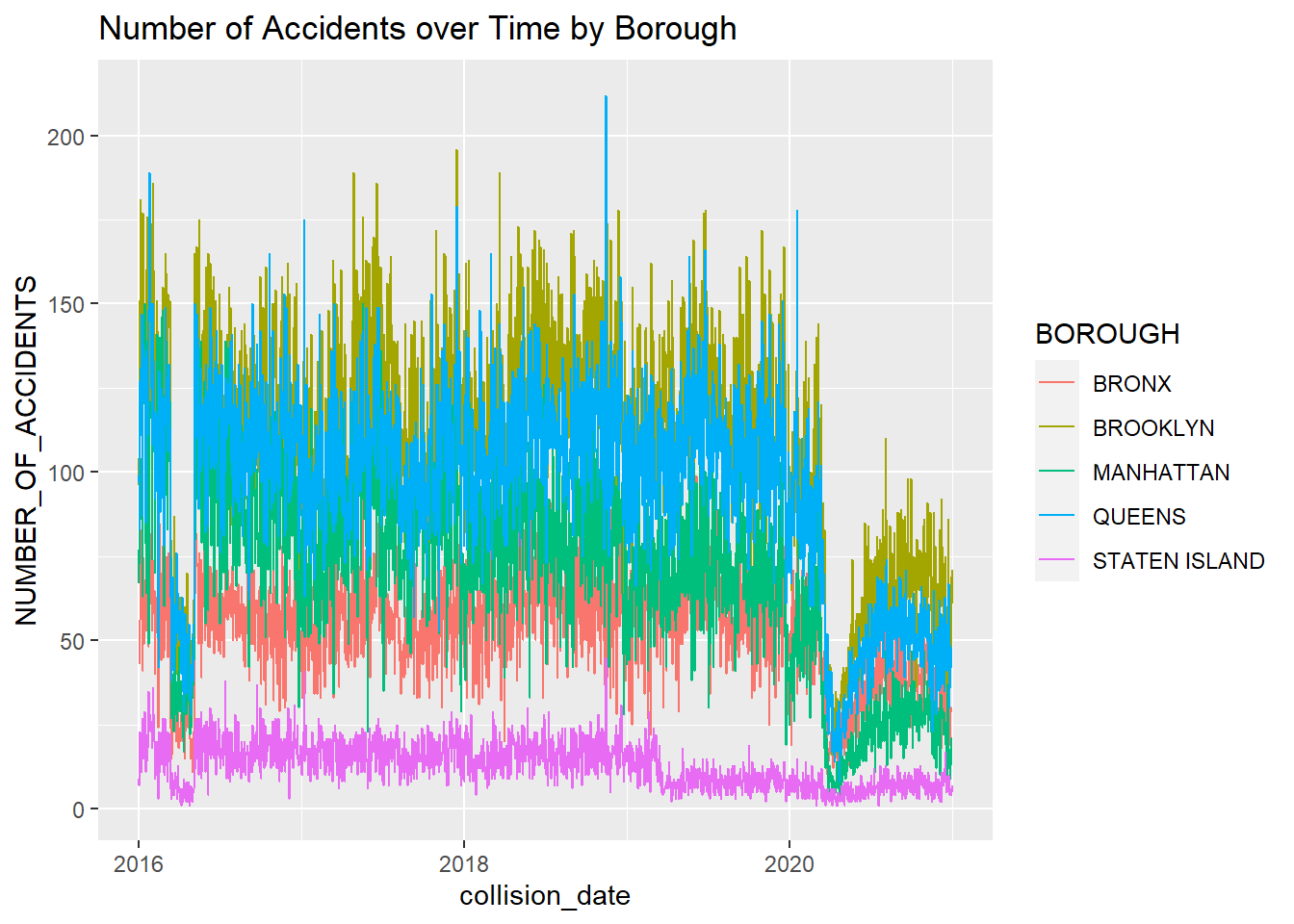
#Missing values exploration
collisions_missing <- collision %>%
  mutate(MISSING_BOROUGH=1*is.na(BOROUGH),
         MISSING_CONTRIBUTION_INFO=1*is.na(`CONTRIBUTING FACTOR VEHICLE 1`)) %>%
         select(MISSING_BOROUGH, MISSING_CONTRIBUTION_INFO, YEAR, BOROUGH)
missing_borough_by_year <- collisions_missing %>%
  group_by(YEAR) %>% summarise(percent_missing_borough=mean(MISSING_BOROUGH))
missing_contrib_by_year <- collisions_missing %>%
  group_by(YEAR) %>% summarise(percent_missing_contrib=mean(MISSING_CONTRIBUTION_INFO))
missing_contrib_by_borough <- collisions_missing %>%
  group_by(BOROUGH)%>%summarise(percent_missing_contrib=mean(MISSING_CONTRIBUTION_INFO))
#Years with the highest missing information
ggplot(data=missing_borough_by_year, aes(x=YEAR, y=percent_missing_borough,)) + geom_col(aes(fill=percent_missing_borough))+
  xlab("Year") + ylab("% Missing Borough Information") +
  ggtitle("% Missing Borough Information vs Year")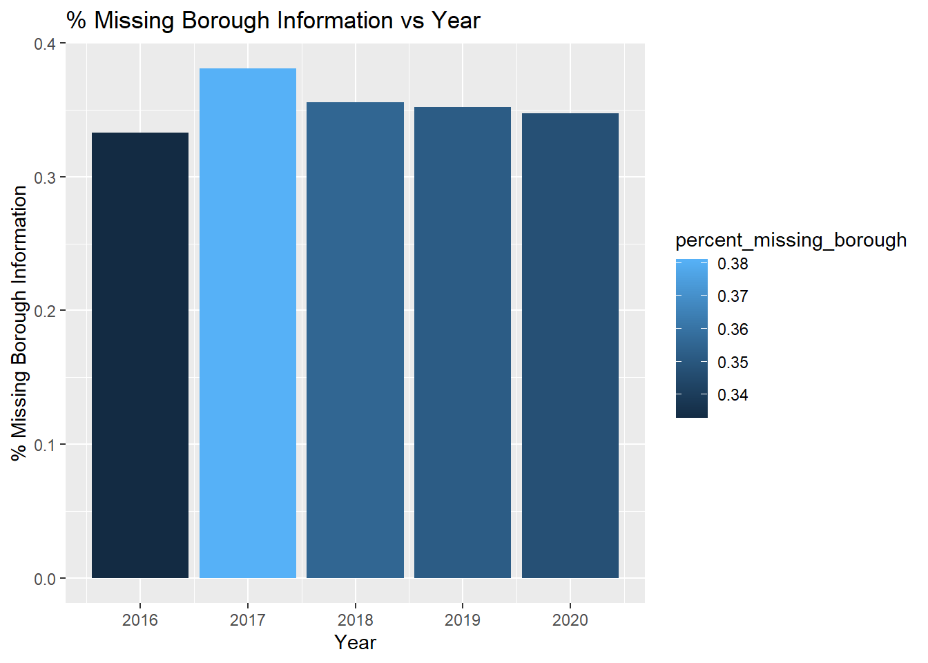
#Variables with highest missing percentage of values
naValues = as.data.frame(100* apply(collision, 2, function(col)sum(is.na(col))/length(col)))
naValues$Var = rownames(naValues)
colnames(naValues) = c("NA_Percentage","Variables")
naValues <- naValues[order(naValues$NA_Percentage),]
ggplot(naValues,aes(y= NA_Percentage, x=reorder( Variables,NA_Percentage)))+
geom_bar( stat="identity", position = "dodge", fill ="red")+
coord_flip()+
theme_classic()+
scale_colour_brewer() +
  scale_y_continuous()+ ggtitle("Percentage of Missing Values in NYC Vehicle Collisions Dataset \nby Variable Type") +ylab("Missing Value Percentage") + xlab("Variables")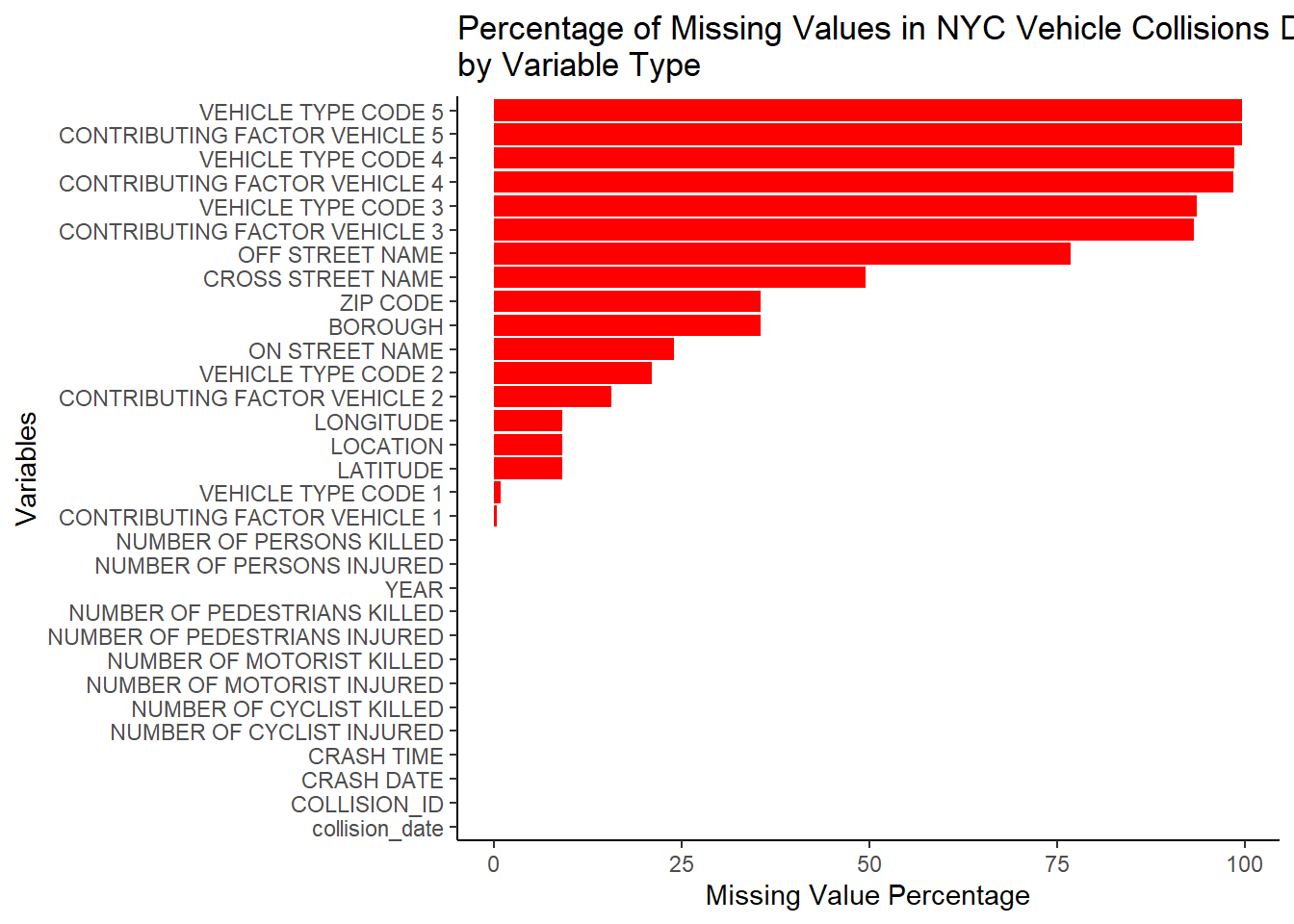
#Accidents in each borough over time.
collision_use['collision_date'] = as.Date(collision_use$DATE, format="%m/%d/%Y")
collision_use<- collision_use%>% mutate(., year = year(collision_date))
collision_use%>% mutate(., year = year(collision_date)) %>%
  group_by(., BOROUGH, year) %>%
  summarise(.,count = n()) %>%
  ggplot(aes(x=year, y=count))+
  geom_line(stat="identity", aes(color=BOROUGH))+geom_point()+ggtitle("Number of Accidents Over Time by Borough") +
  scale_colour_viridis_d("plasma")
## `summarise()` has grouped output by 'BOROUGH'. You can override using the `.groups` argument.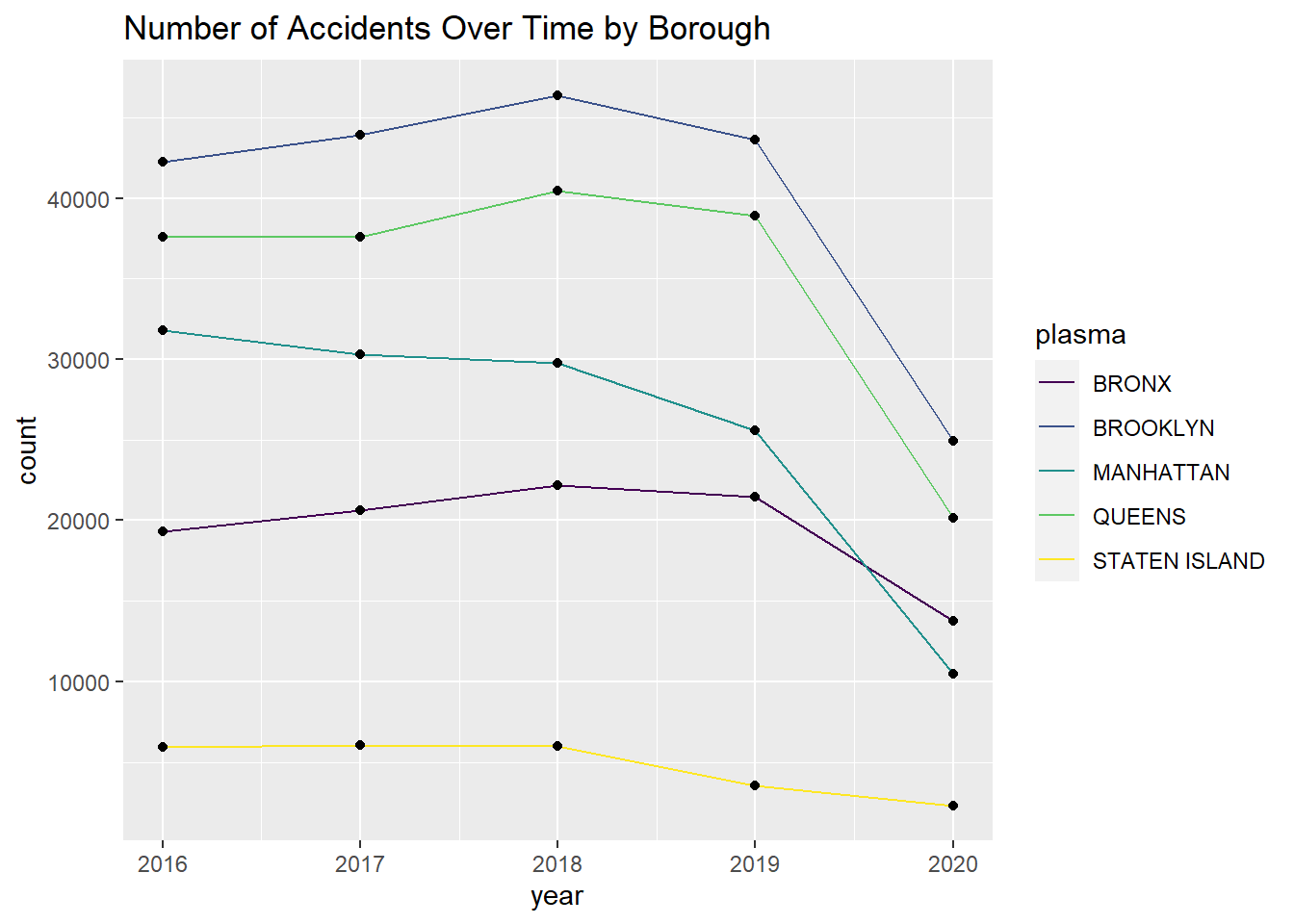
#CONTRIBUTING FACTOR EDA
print("Number of missing values in `CONTRIBUTING FACTOR VEHICLE 1`")
## [1] "Number of missing values in `CONTRIBUTING FACTOR VEHICLE 1`"print(sum(is.na(collision_use$`CONTRIBUTING FACTOR VEHICLE 1`)))## [1] 2429print("Number of missing values in `CONTRIBUTING FACTOR VEHICLE 2`")## [1] "Number of missing values in `CONTRIBUTING FACTOR VEHICLE 2`"print(sum(is.na(collision_use$`CONTRIBUTING FACTOR VEHICLE 2`)))## [1] 106742#ma
#Top 10 contributing factors for Vehicle 1
collisions_by_factor1 <- collision_use%>% filter(!is.na(`CONTRIBUTING FACTOR VEHICLE 1`)) %>%
filter(`CONTRIBUTING FACTOR VEHICLE 1` != "Unspecified") %>%
group_by(`CONTRIBUTING FACTOR VEHICLE 1`) %>%
summarise(NUMBER_OF_ACCIDENTS=n(),
NUMBER_OF_DEATHS = sum(`NUMBER OF PERSONS KILLED`)) %>%
arrange(desc(NUMBER_OF_ACCIDENTS))
collisions_by_factor1 <- head(collisions_by_factor1, n = 10)
ggplot(collisions_by_factor1, aes(x=reorder(`CONTRIBUTING FACTOR VEHICLE 1`, `NUMBER_OF_ACCIDENTS`, fill=`CONTRIBUTING FACTOR VEHICLE 1`), y=`NUMBER_OF_ACCIDENTS`))+
geom_col(aes(fill=`CONTRIBUTING FACTOR VEHICLE 1`))+
ggtitle("Top 10 First Contributing Factors by Accident Count")+
xlab("Contributing Factor Vehicle 1")+
ylab("Number of Accidents")+
coord_flip()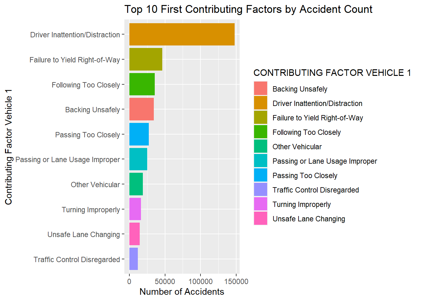
collisions_by_factor2 <- collision_use%>% filter(!is.na(`CONTRIBUTING FACTOR VEHICLE 2`)) %>%
  filter(`CONTRIBUTING FACTOR VEHICLE 2` != "Unspecified") %>%
  group_by(`CONTRIBUTING FACTOR VEHICLE 2`) %>%
  summarise(NUMBER_OF_ACCIDENTS=n(),
            NUMBER_OF_DEATHS = sum(`NUMBER OF PERSONS KILLED`)) %>%
  arrange(desc(NUMBER_OF_ACCIDENTS))
collisions_by_factor2 <- head(collisions_by_factor2, n = 10)


ggplot(collisions_by_factor2, aes(x=reorder(`CONTRIBUTING FACTOR VEHICLE 2`, `NUMBER_OF_ACCIDENTS`, fill=`CONTRIBUTING FACTOR VEHICLE 2`), y=`NUMBER_OF_ACCIDENTS`))+
geom_col(aes(fill=`CONTRIBUTING FACTOR VEHICLE 2`))+
ggtitle("Top 10 Second Contributing Factors by Accident Count")+
xlab("Contributing Factor Vehicle 2")+
ylab("Number of Accidents")+
coord_flip()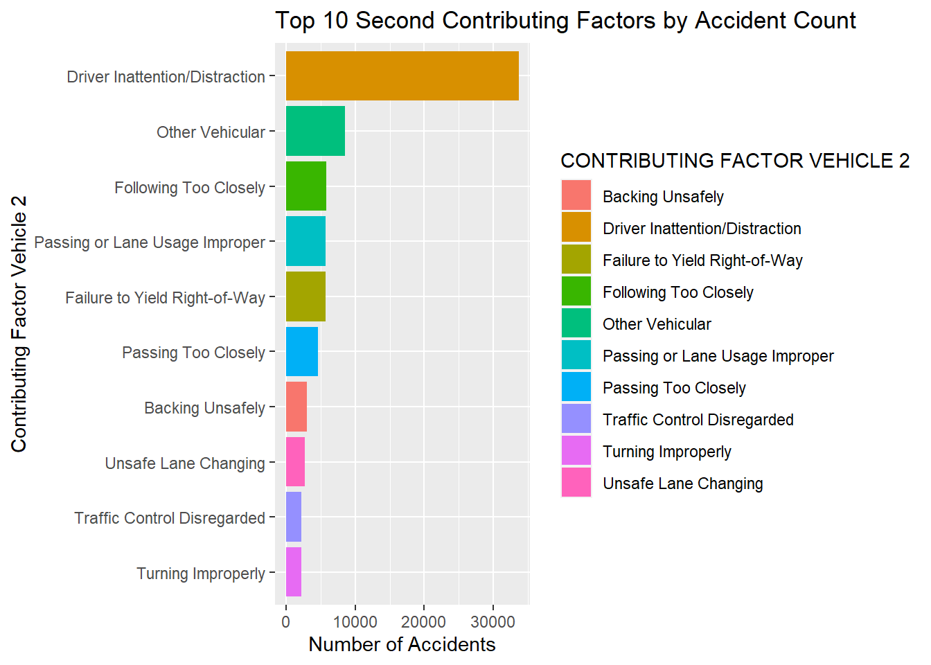
#Vehicle Type EDA
#Most of the observations do not have variables `CONTRIBUTING FACTOR VEHICLE 5`, `VEHICLE TYPE CODE 5` etc, I dropped them, and Created a new binary variable which represents if 3 or more vehicles were involved in an accident.
collision_use <- collision_use %>% mutate(VEHICLES_INVOLVED_GTE3 = 1 * !is.na(`CONTRIBUTING FACTOR VEHICLE 3`))
collision_use <- collision_use %>% select(-c(`VEHICLE TYPE CODE 5`,`CONTRIBUTING FACTOR VEHICLE 5`,
                                     `VEHICLE TYPE CODE 4`,`CONTRIBUTING FACTOR VEHICLE 4`,
                                     `VEHICLE TYPE CODE 3`,`CONTRIBUTING FACTOR VEHICLE 3`,
                                     ))
#Number of Accidents and Number of Deaths for Combinations of Vehicle Types 1 and 2.
collision_by_vehicleTypes <- collision_use %>%
  filter(!is.na(`VEHICLE TYPE CODE 1`) & !is.na(`VEHICLE TYPE CODE 2`)) %>%
  filter(`VEHICLE TYPE CODE 1` != "UNKNOWN" & `VEHICLE TYPE CODE 2` != "UNKNOWN") %>%
  group_by(`VEHICLE TYPE CODE 1`,`VEHICLE TYPE CODE 2`) %>%
  summarise(NUMBER_OF_ACCIDENTS=n(),
            NUMBER_OF_DEATHS = sum(`NUMBER OF PERSONS KILLED`)) %>%
  arrange(desc(NUMBER_OF_ACCIDENTS))
## `summarise()` has grouped output by 'VEHICLE TYPE CODE 1'. You can override using the `.groups` argument.#Injuries/Deaths of person type by borough
collision_persontype <- collision_use %>% group_by(BOROUGH) %>% summarise(Ped_Injuries = sum(`NUMBER OF PEDESTRIANS INJURED`), Ped_Deaths = sum(`NUMBER OF PEDESTRIANS KILLED`), Cyclist_Injuries = sum(`NUMBER OF CYCLIST INJURED`), Cyclist_Deaths = sum(`NUMBER OF CYCLIST KILLED`), Motorist_Injuries = sum(`NUMBER OF MOTORIST INJURED`), Motorist_Deaths = sum(`NUMBER OF MOTORIST KILLED`)) %>% mutate(Ped_Fatality_Rate=Ped_Deaths/Ped_Injuries, Cyclist_Fatality_Rate=Cyclist_Deaths/Cyclist_Injuries, Motorist_Fatality_Rate=Motorist_Deaths/Motorist_Injuries)
df1 <- data.frame(collision_persontype$Ped_Fatality_Rate, collision_persontype$Cyclist_Fatality_Rate, collision_persontype$Motorist_Fatality_Rate, collision_persontype$BOROUGH)
df2 <- tidyr::pivot_longer(df1, cols=c('collision_persontype.Ped_Fatality_Rate', 'collision_persontype.Cyclist_Fatality_Rate', 'collision_persontype.Motorist_Fatality_Rate'), names_to='Type',
values_to="Fatality_Rate")
ggplot(df2, aes(x=collision_persontype.BOROUGH, y=Fatality_Rate, fill=Type)) +
geom_bar(stat='identity', position='dodge')+ggtitle('Borough Fatality Rates by Person Type')+ xlab('Borough')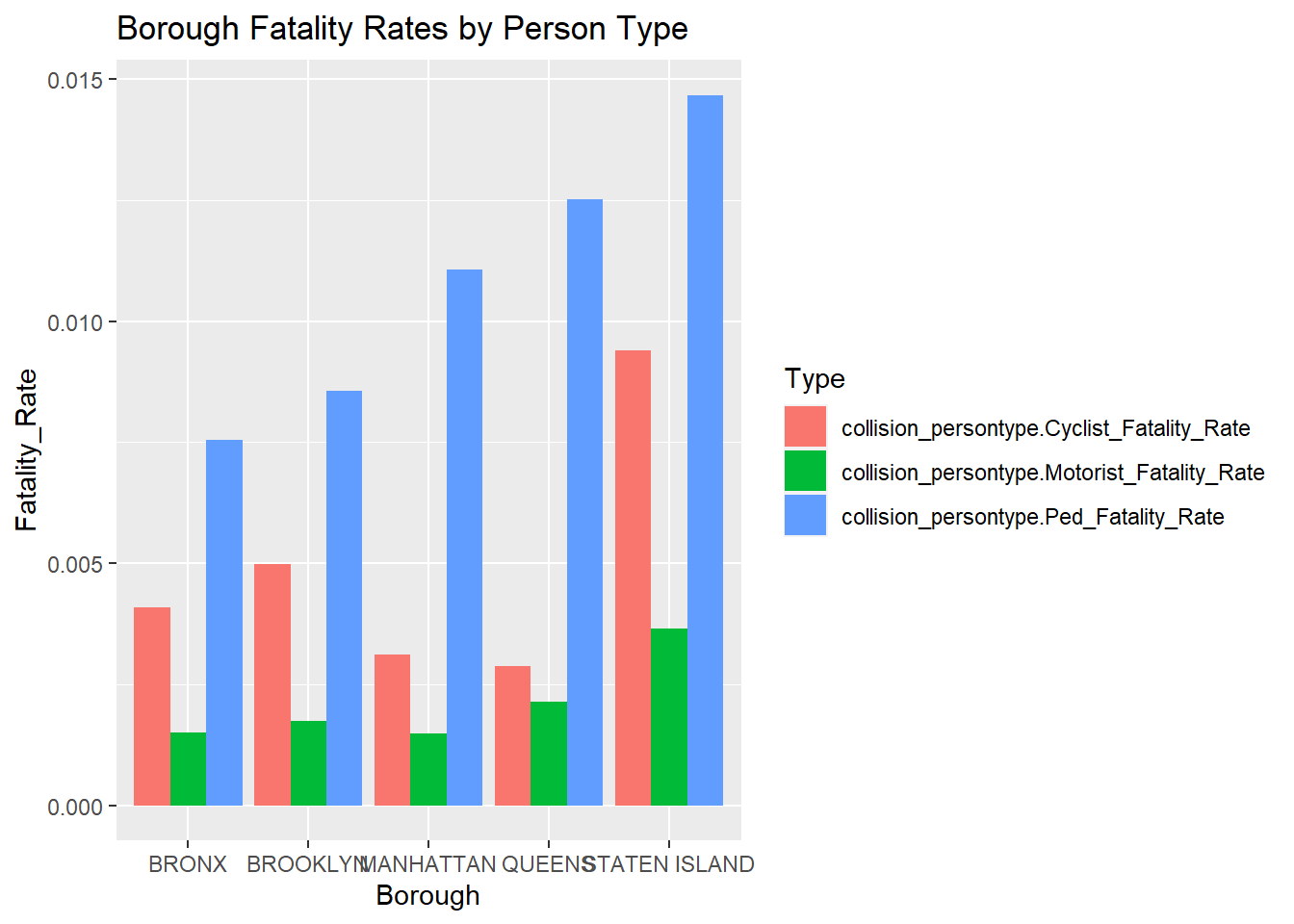
collision_10000 <- collision %>% separate(`CRASH DATE`, c("MONTH", "DAY", "YEAR"), sep = "/")  %>% sample_n(10000) %>% filter(YEAR != 2012, YEAR != 2015, YEAR != 2013, YEAR != 2014) %>% write_csv("NYC Collision 10000.csv")


collision_use <- collision %>%
  filter(!is.na(BOROUGH), !is.na('ZIP CODE'), !is.na(LONGITUDE), !is.na(LATITUDE), !is.na(LOCATION), !is.na(`NUMBER OF PEDESTRIANS KILLED`), !is.na(`NUMBER OF CYCLIST INJURED`)) %>% select(-(`ON STREET NAME`:`OFF STREET NAME`)) %>%
  rename(DATE = `CRASH DATE`, TIME = `CRASH TIME`, ZIPCODE = `ZIP CODE`, LOCATION = `LOCATION`) %>% separate(DATE, c("MONTH", "DAY", "YEAR"), sep = "/") %>%
  separate(TIME, c("HOUR", "MINUTE"), sep = ":") %>%
  mutate(`CONTRIBUTING FACTOR VEHICLE 1` = str_to_lower(`CONTRIBUTING FACTOR VEHICLE 1`)) %>%
   mutate(`CONTRIBUTING FACTOR VEHICLE 2` = str_to_lower(`CONTRIBUTING FACTOR VEHICLE 2`)) %>%
   mutate(`CONTRIBUTING FACTOR VEHICLE 3` = str_to_lower(`CONTRIBUTING FACTOR VEHICLE 3`)) %>%
   mutate(`CONTRIBUTING FACTOR VEHICLE 4` = str_to_lower(`CONTRIBUTING FACTOR VEHICLE 4`)) %>%
   mutate(`CONTRIBUTING FACTOR VEHICLE 5` = str_to_lower(`CONTRIBUTING FACTOR VEHICLE 5`)) %>% filter(!is.na(`CONTRIBUTING FACTOR VEHICLE 1`),!is.na(`CONTRIBUTING FACTOR VEHICLE 2`), !is.na(`CONTRIBUTING FACTOR VEHICLE 3`), !is.na(`CONTRIBUTING FACTOR VEHICLE 4`), !is.na(`CONTRIBUTING FACTOR VEHICLE 5`)) %>% pivot_longer(`CONTRIBUTING FACTOR VEHICLE 1`:`CONTRIBUTING FACTOR VEHICLE 5`, names_to = "CONTRIBUTING VEHICLE", values_to = "CAUSE") %>% filter(!is.na(CAUSE)) %>%
  pivot_longer(`VEHICLE TYPE CODE 1`:`VEHICLE TYPE CODE 5`, names_to = "VEHICLE CODE", values_to = "VEHICLE") %>% select(-(`CONTRIBUTING VEHICLE`)) %>% select(-(`VEHICLE CODE`)) %>% mutate(VEHICLE = str_to_lower(VEHICLE)) %>%
  sample_n(1000) %>%
  filter(!is.na("VEHICLE"))

collision_use
## # A tibble: 1,000 x 22
## MONTH DAY YEAR HOUR MINUTE BOROUGH ZIPCODE LATITUDE LONGITUDE LOCATION
## <chr> <chr> <chr> <chr> <chr> <chr> <dbl> <dbl> <dbl> <chr>
## 1 02 24 2016 13 00 BROOKLYN 11208 40.7 -73.9 (40.65886~
## 2 07 13 2017 21 45 BROOKLYN 11231 40.7 -74.0 (40.67769~
## 3 01 15 2020 22 10 QUEENS 11420 40.7 -73.8 (40.68302~
## 4 05 20 2019 8 30 QUEENS 11377 40.7 -73.9 (40.7497,~
## 5 06 11 2016 10 30 STATEN ~ 10307 40.5 -74.2 (40.51393~
## 6 03 10 2018 6 00 QUEENS 11434 40.7 -73.8 (40.68139~
## 7 06 26 2016 12 20 QUEENS 11105 40.8 -73.9 (40.78045~
## 8 06 24 2017 3 00 QUEENS 11429 40.7 -73.7 (40.70316~
## 9 08 27 2020 16 10 QUEENS 11419 40.7 -73.8 (40.68868~
## 10 03 05 2016 11 00 QUEENS 11368 40.8 -73.9 (40.75718~
## # ... with 990 more rows, and 12 more variables:
## # NUMBER OF PERSONS INJURED <dbl>, NUMBER OF PERSONS KILLED <dbl>,
## # NUMBER OF PEDESTRIANS INJURED <dbl>, NUMBER OF PEDESTRIANS KILLED <dbl>,
## # NUMBER OF CYCLIST INJURED <dbl>, NUMBER OF CYCLIST KILLED <dbl>,
## # NUMBER OF MOTORIST INJURED <dbl>, NUMBER OF MOTORIST KILLED <dbl>,
## # COLLISION_ID <dbl>, collision_date <date>, CAUSE <chr>, VEHICLE <chr>Number of Accidents by Borough and Vehicle Type:
collision_use %>% group_by(VEHICLE) %>% ggplot(aes(x = VEHICLE, y = stat(prop), group = 1)) + geom_bar() + facet_wrap(~BOROUGH)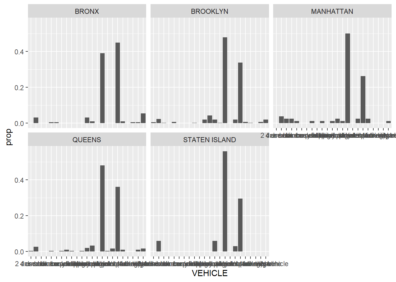
Number of Accidents by Month(Time of the Year):
collision_use %>% group_by(MONTH) %>% mutate(count = n()) %>% ggplot(aes(x = MONTH, y = count, group = 1)) + geom_line(aes(color = BOROUGH))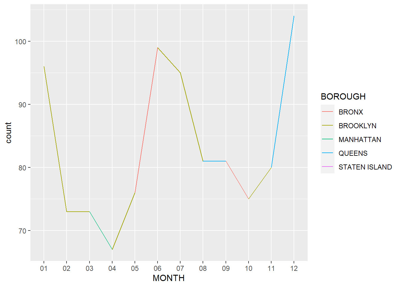
Number of Accidents by Hour (Time of the Day):
collision_use %>% group_by(HOUR) %>% filter(HOUR <= 24) %>% summarize(count = n()) %>% ggplot(aes(x = HOUR, y = count, group = 1)) + geom_line()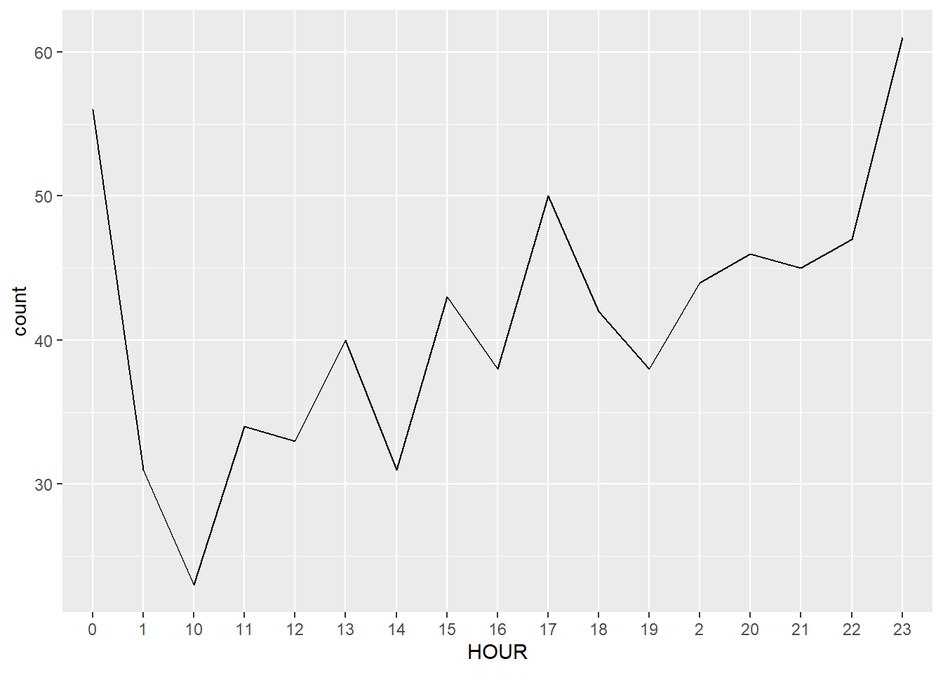
Number of Person’s Injured by Borough:
collision_use %>% ggplot(aes(x = BOROUGH, y = `NUMBER OF PERSONS INJURED`)) + geom_col()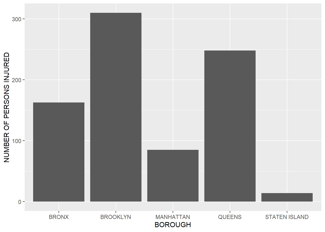
Number of Pedestrians Injured by Borough:
collision_use %>% ggplot(aes(x = BOROUGH, y = `NUMBER OF PEDESTRIANS KILLED`)) + geom_col()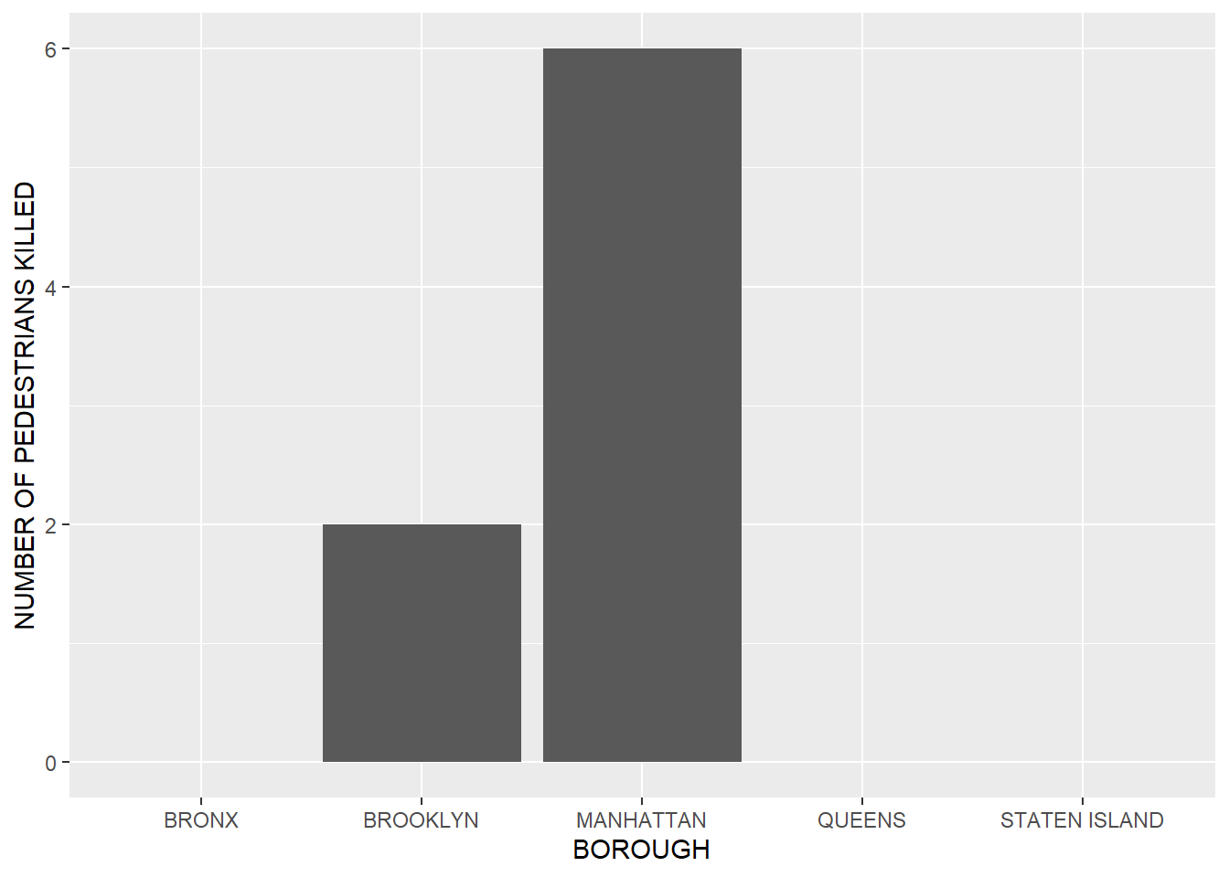 Number of Cyclists Injured by Borough:
collision_use %>% ggplot(aes(x = BOROUGH, y = `NUMBER OF CYCLIST INJURED`)) + geom_col()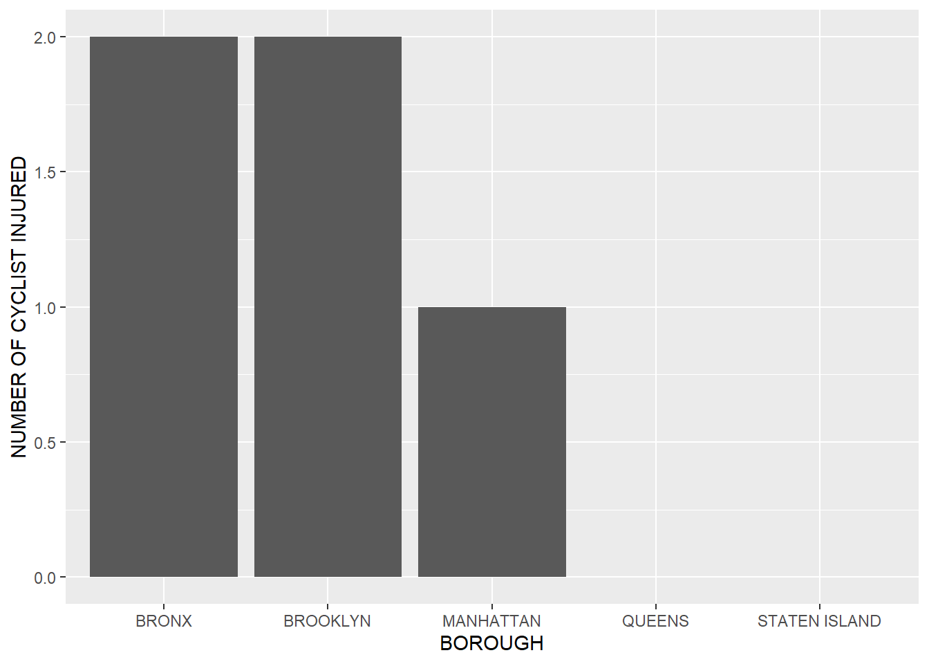
collision_use %>% group_by(CAUSE) %>% mutate(count = n()) %>% ggplot(aes(x = CAUSE, y = count, color = BOROUGH)) + geom_col()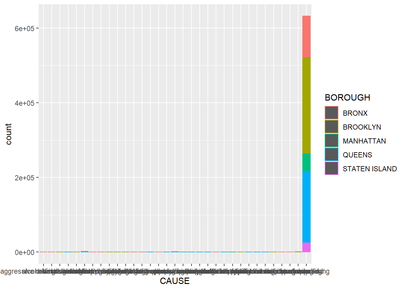
Further Findings (NYC Collisions Data):
Brooklyn, Queens, and Manhattan have the highest proportions of traffic accidents in New York Ciy. The time of the year when traffic accidents seem to peak is during the summer months of June to October. Interestingly, even though the warmer weather might cause an increase in traffic movement which could potentially lead to an increase traffic collisions, there is a sudden drop in April of traffic accidents. During the day, the most traffic accidents were reported at 4pm and is the lowest at 1am to 2am. Furthermore, in terms of vehicle types, my assumption that sedans were the most prevalent type to be involved in accidents proved true.
In terms of causalities and injuries, my initial assumption that was proven correct where Brooklyn, Manhattan, and Queens have the highest number of people injured and pedestrians killed out of the 5 boroughs.
In terms of the cause of accidents, “unspecified” is the most popular contributing reason for accidents in New York City. Rather than ignoring this, it could either mean that there are certain flaws in the data collecting process that could be improved upon, or there is a wide variety of reasons that the standard choices to do not encompass. There is a possibility that it is a combination of both but I believe this is something that should not be ignored.
Other trends: -Looking at the volume of accidents by year affirms our initial prediction that 2020 would experience a severe drop in accidents as COVID and quarantine would limit overall driving/traffic in NYC. -Brooklyn leads all boroughs with the most accidents per year across 5 years, while Staten Island consistently has the least. -Staten Island also has the lowest population density by far. -Driver Inattention and Distraction is the largest driver of accidents in NYC. -Approximately 183,000 accidents have cited this as a contributing factor -Next highest is Failure to Yield Right-of-Way, with approximately 53,000 accidents. -Staten Island experiences the highest Death to Injury ratio among the boroughs across all types of people. Bronx sees a considerably high death rate for cyclists compared to other boroughs. -Sedans seem to be involved in the most accidents, with 7 out of the top 10 vehicle code combinations involving sedans. -Combinations with the most collisions are sedans with other sedans, approximately 95,000 accidents.