#Loading and Cleaning:
library(tidyverse)## -- Attaching packages --------------------------------------- tidyverse 1.3.1 --## v ggplot2 3.3.5 v purrr 0.3.4
## v tibble 3.1.4 v dplyr 1.0.7
## v tidyr 1.1.3 v stringr 1.4.0
## v readr 2.0.1 v forcats 0.5.1## -- Conflicts ------------------------------------------ tidyverse_conflicts() --
## x dplyr::filter() masks stats::filter()
## x dplyr::lag() masks stats::lag()library(dplyr)
library(lubridate)##
## Attaching package: 'lubridate'## The following objects are masked from 'package:base':
##
## date, intersect, setdiff, unioncollision <- read_csv(here::here('dataset/NYC Collision Data.csv'))## Rows: 1831755 Columns: 29## -- Column specification --------------------------------------------------------
## Delimiter: ","
## chr (17): CRASH DATE, CRASH TIME, BOROUGH, LOCATION, ON STREET NAME, CROSS S...
## dbl (12): ZIP CODE, LATITUDE, LONGITUDE, NUMBER OF PERSONS INJURED, NUMBER O...##
## i Use `spec()` to retrieve the full column specification for this data.
## i Specify the column types or set `show_col_types = FALSE` to quiet this message.collision['collision_date'] = as.Date(collision$'CRASH DATE', format="%m/%d/%Y")
collision<- collision%>%mutate(., YEAR = year(collision_date))
collision<- collision%>%filter(YEAR>2015 & YEAR<2021)
summary(collision)## CRASH DATE CRASH TIME BOROUGH ZIP CODE
## Length:1016774 Length:1016774 Length:1016774 Min. :10000
## Class :character Class :character Class :character 1st Qu.:10451
## Mode :character Mode :character Mode :character Median :11208
## Mean :10859
## 3rd Qu.:11249
## Max. :11697
## NA's :360780
## LATITUDE LONGITUDE LOCATION ON STREET NAME
## Min. : 0.00 Min. :-201.36 Length:1016774 Length:1016774
## 1st Qu.:40.67 1st Qu.: -73.97 Class :character Class :character
## Median :40.72 Median : -73.92 Mode :character Mode :character
## Mean :40.67 Mean : -73.83
## 3rd Qu.:40.77 3rd Qu.: -73.86
## Max. :43.34 Max. : 0.00
## NA's :92548 NA's :92548
## CROSS STREET NAME OFF STREET NAME NUMBER OF PERSONS INJURED
## Length:1016774 Length:1016774 Min. : 0.0000
## Class :character Class :character 1st Qu.: 0.0000
## Mode :character Mode :character Median : 0.0000
## Mean : 0.2841
## 3rd Qu.: 0.0000
## Max. :31.0000
## NA's :17
## NUMBER OF PERSONS KILLED NUMBER OF PEDESTRIANS INJURED
## Min. :0.000000 Min. : 0.00000
## 1st Qu.:0.000000 1st Qu.: 0.00000
## Median :0.000000 Median : 0.00000
## Mean :0.001224 Mean : 0.04979
## 3rd Qu.:0.000000 3rd Qu.: 0.00000
## Max. :8.000000 Max. :27.00000
## NA's :31
## NUMBER OF PEDESTRIANS KILLED NUMBER OF CYCLIST INJURED
## Min. :0.000000 Min. :0.00000
## 1st Qu.:0.000000 1st Qu.:0.00000
## Median :0.000000 Median :0.00000
## Mean :0.000621 Mean :0.02474
## 3rd Qu.:0.000000 3rd Qu.:0.00000
## Max. :6.000000 Max. :3.00000
##
## NUMBER OF CYCLIST KILLED NUMBER OF MOTORIST INJURED NUMBER OF MOTORIST KILLED
## Min. :0.0000000 Min. : 0.0000 Min. :0.000000
## 1st Qu.:0.0000000 1st Qu.: 0.0000 1st Qu.:0.000000
## Median :0.0000000 Median : 0.0000 Median :0.000000
## Mean :0.0001131 Mean : 0.2094 Mean :0.000488
## 3rd Qu.:0.0000000 3rd Qu.: 0.0000 3rd Qu.:0.000000
## Max. :2.0000000 Max. :31.0000 Max. :4.000000
##
## CONTRIBUTING FACTOR VEHICLE 1 CONTRIBUTING FACTOR VEHICLE 2
## Length:1016774 Length:1016774
## Class :character Class :character
## Mode :character Mode :character
##
##
##
##
## CONTRIBUTING FACTOR VEHICLE 3 CONTRIBUTING FACTOR VEHICLE 4
## Length:1016774 Length:1016774
## Class :character Class :character
## Mode :character Mode :character
##
##
##
##
## CONTRIBUTING FACTOR VEHICLE 5 COLLISION_ID VEHICLE TYPE CODE 1
## Length:1016774 Min. :3363355 Length:1016774
## Class :character 1st Qu.:3618219 Class :character
## Mode :character Median :3872688 Mode :character
## Mean :3872628
## 3rd Qu.:4127036
## Max. :4463721
##
## VEHICLE TYPE CODE 2 VEHICLE TYPE CODE 3 VEHICLE TYPE CODE 4
## Length:1016774 Length:1016774 Length:1016774
## Class :character Class :character Class :character
## Mode :character Mode :character Mode :character
##
##
##
##
## VEHICLE TYPE CODE 5 collision_date YEAR
## Length:1016774 Min. :2016-01-01 Min. :2016
## Class :character 1st Qu.:2017-02-13 1st Qu.:2017
## Mode :character Median :2018-03-22 Median :2018
## Mean :2018-04-02 Mean :2018
## 3rd Qu.:2019-05-05 3rd Qu.:2019
## Max. :2020-12-31 Max. :2020
## collision_use <- collision %>% filter(!is.na(BOROUGH), !is.na('ZIP CODE'), !is.na(LONGITUDE), !is.na(LATITUDE), !is.na(LOCATION))%>% select(-(`ON STREET NAME`:`OFF STREET NAME`)) %>%
rename(DATE = `CRASH DATE`, TIME = `CRASH TIME`, ZIPCODE = `ZIP CODE`, LOCATION = `LOCATION`)
collision_use['collision_date'] = as.Date(collision_use$DATE, format="%m/%d/%Y")
collision_use<- collision_use%>% mutate(., year = year(collision_date))
collision_use$TIME<- as.character(collision_use$TIME)
collision_use$TIME <- as.numeric(unlist(strsplit(collision_use$TIME, ":"))[seq(1, 2 * nrow(collision_use), 2)])#EDA
collisions_per_day <-collision_use %>%
group_by(collision_date, BOROUGH) %>%
summarise(NUMBER_OF_ACCIDENTS=n(),
NUMBER_OF_DEATHS = sum(`NUMBER OF PERSONS KILLED`),
NUMBER_OF_INJURIES = sum(`NUMBER OF PERSONS INJURED`))%>%
ungroup()## `summarise()` has grouped output by 'collision_date'. You can override using the `.groups` argument.ggplot(data=collisions_per_day, aes(x=collision_date, y=NUMBER_OF_ACCIDENTS))+
geom_line(aes(group=BOROUGH, color=BOROUGH))+ggtitle("Figure 1: Number of Accidents over Time by Borough")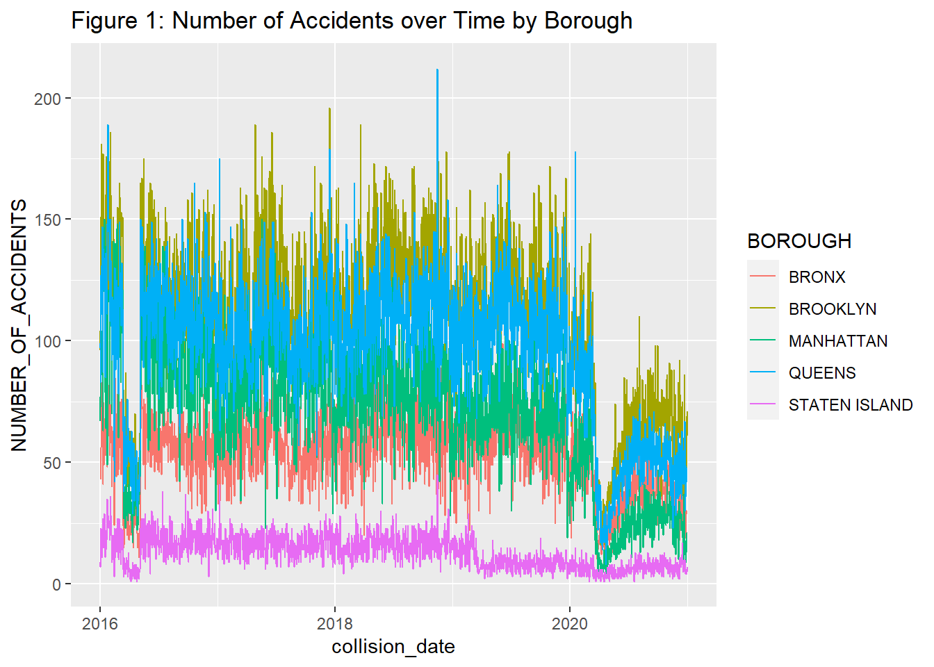 In Figure 1, we observe that if we take the data set as it is from 2016-2020, the highest number of accidents occur in Brooklyn and the lowest number of accidents occur in Staten Island. This potentially could be because of the narrow roads in Brooklyn and not much population or vehicles in Staten Island. We will now clean the data set and and revisit this to see if our results change in anyway. It is also noteworthy that there is an overall decrease in number of accidents in mid 2016 and early 2020. It could be interesting to see what could be the reasons for that in 2016 and in 2020, we assume that the decrease is caused due to the pandemic.
#Missing values exploration
collisions_missing <- collision %>%
mutate(MISSING_BOROUGH=1*is.na(BOROUGH),
MISSING_CONTRIBUTION_INFO=1*is.na(`CONTRIBUTING FACTOR VEHICLE 1`)) %>%
select(MISSING_BOROUGH, MISSING_CONTRIBUTION_INFO, YEAR, BOROUGH)
missing_borough_by_year <- collisions_missing %>%
group_by(YEAR) %>% summarise(percent_missing_borough=mean(MISSING_BOROUGH))
missing_contrib_by_year <- collisions_missing %>%
group_by(YEAR) %>% summarise(percent_missing_contrib=mean(MISSING_CONTRIBUTION_INFO))
missing_contrib_by_borough <- collisions_missing %>%
group_by(BOROUGH)%>%summarise(percent_missing_contrib=mean(MISSING_CONTRIBUTION_INFO))In the following two plots, we will understand the data a little more to see what is relevant to look at and what is not. The plot “Percentage of Missing Values in NYC Vehicle Collisions Dataset by Variable Type” tells us how many missing values are there for each variable and we can easily remove the ones which have 0 to few values that are relevant.
#Years with the highest missing information
ggplot(data=missing_borough_by_year, aes(x=YEAR, y=percent_missing_borough,)) + geom_col(aes(fill=percent_missing_borough))+
xlab("Year") + ylab("% Missing Borough Information") +
ggtitle("% Missing Borough Information per Year")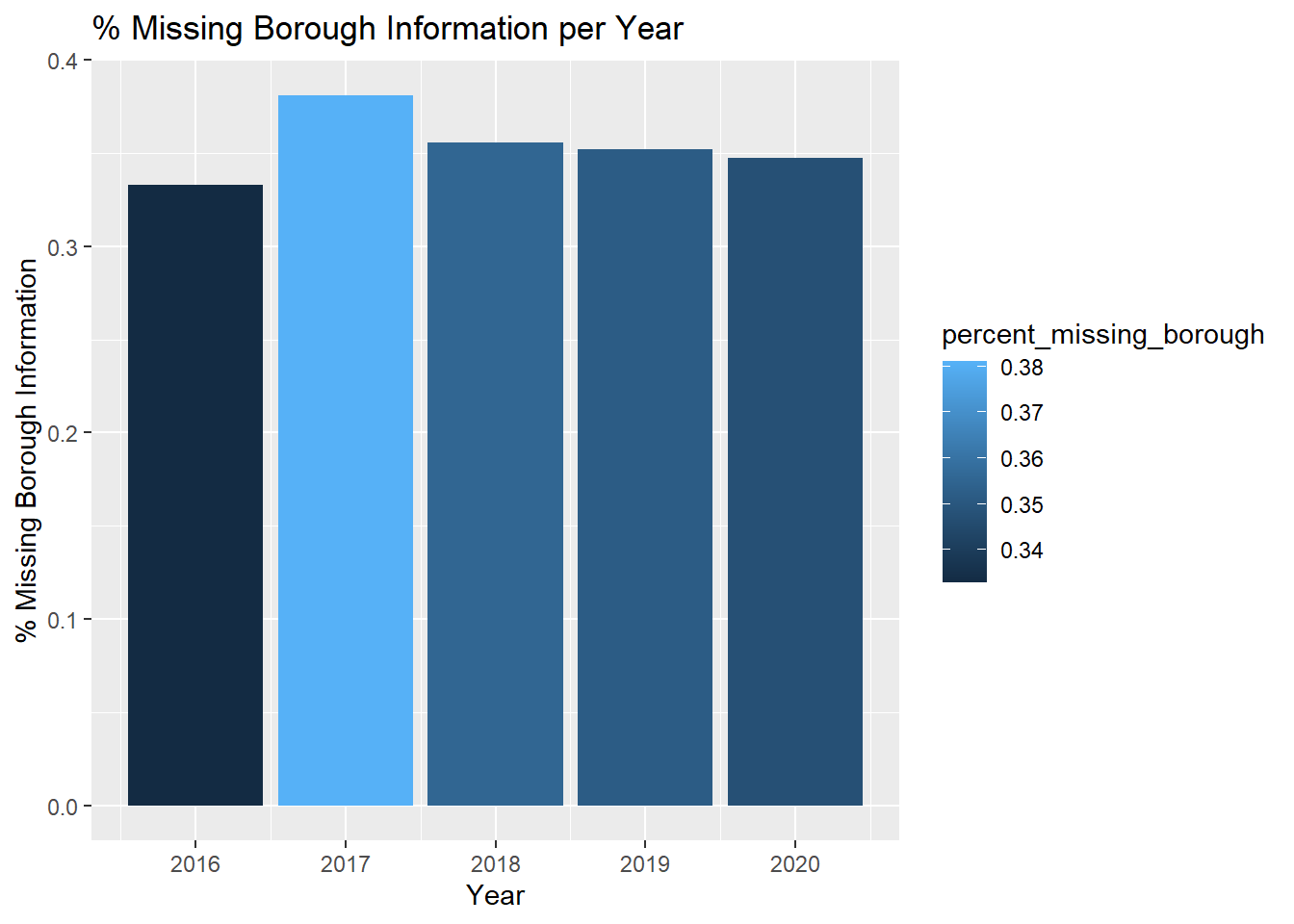
#Variables with highest missing percentage of values
naValues = as.data.frame(100* apply(collision, 2, function(col)sum(is.na(col))/length(col)))
naValues$Var = rownames(naValues)
colnames(naValues) = c("NA_Percentage","Variables")
naValues <- naValues[order(naValues$NA_Percentage),]
ggplot(naValues,aes(y= NA_Percentage, x=reorder( Variables,NA_Percentage)))+
geom_bar( stat="identity", position = "dodge", fill ="red")+
coord_flip()+
theme_classic()+
scale_colour_brewer() +
scale_y_continuous()+ ggtitle("Percentage of Missing Values in NYC Vehicle Collisions Dataset \nby Variable Type") +ylab("Missing Value Percentage") + xlab("Variables")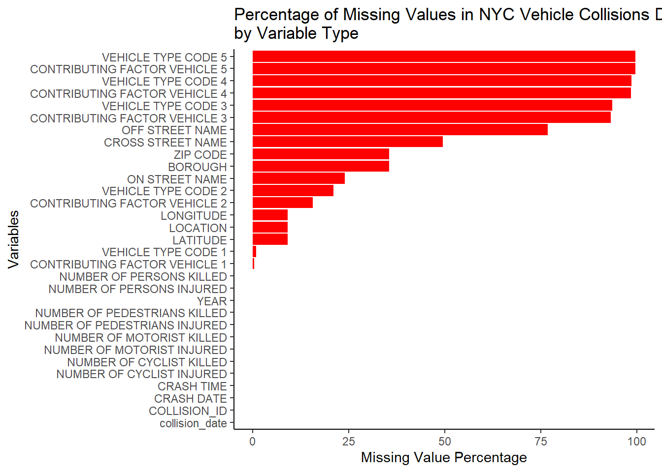
#CONTRIBUTING FACTOR EDA
print("Number of missing values in `CONTRIBUTING FACTOR VEHICLE 1`")## [1] "Number of missing values in `CONTRIBUTING FACTOR VEHICLE 1`"print(sum(is.na(collision_use$`CONTRIBUTING FACTOR VEHICLE 1`)))## [1] 2429print("Number of missing values in `CONTRIBUTING FACTOR VEHICLE 2`")## [1] "Number of missing values in `CONTRIBUTING FACTOR VEHICLE 2`"print(sum(is.na(collision_use$`CONTRIBUTING FACTOR VEHICLE 2`)))## [1] 106742#Top 10 contributing factors for Vehicle 1
collisions_by_factor1 <- collision_use%>% filter(!is.na(`CONTRIBUTING FACTOR VEHICLE 1`)) %>%
filter(`CONTRIBUTING FACTOR VEHICLE 1` != "Unspecified") %>%
group_by(`CONTRIBUTING FACTOR VEHICLE 1`) %>%
summarise(NUMBER_OF_ACCIDENTS=n(),
NUMBER_OF_DEATHS = sum(`NUMBER OF PERSONS KILLED`)) %>%
arrange(desc(NUMBER_OF_ACCIDENTS))
collisions_by_factor1 <- head(collisions_by_factor1, n = 10)
ggplot(collisions_by_factor1, aes(x=reorder(`CONTRIBUTING FACTOR VEHICLE 1`, `NUMBER_OF_ACCIDENTS`, fill=`CONTRIBUTING FACTOR VEHICLE 1`), y=`NUMBER_OF_ACCIDENTS`))+
geom_col(aes(fill=`CONTRIBUTING FACTOR VEHICLE 1`))+
ggtitle("Top 10 First Contributing Factors by Accident Count")+
xlab("Contributing Factor Vehicle 1")+
ylab("Number of Accidents")+
coord_flip()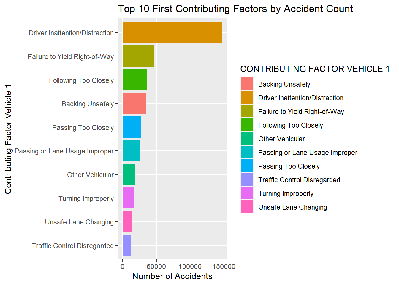
collisions_by_factor2 <- collision_use%>% filter(!is.na(`CONTRIBUTING FACTOR VEHICLE 2`)) %>%
filter(`CONTRIBUTING FACTOR VEHICLE 2` != "Unspecified") %>%
group_by(`CONTRIBUTING FACTOR VEHICLE 2`) %>%
summarise(NUMBER_OF_ACCIDENTS=n(),
NUMBER_OF_DEATHS = sum(`NUMBER OF PERSONS KILLED`)) %>%
arrange(desc(NUMBER_OF_ACCIDENTS))
collisions_by_factor2 <- head(collisions_by_factor2, n = 10)
ggplot(collisions_by_factor2, aes(x=reorder(`CONTRIBUTING FACTOR VEHICLE 2`, `NUMBER_OF_ACCIDENTS`, fill=`CONTRIBUTING FACTOR VEHICLE 2`), y=`NUMBER_OF_ACCIDENTS`))+
geom_col(aes(fill=`CONTRIBUTING FACTOR VEHICLE 2`))+
ggtitle("Top 10 Second Contributing Factors by Accident Count")+
xlab("Contributing Factor Vehicle 2")+
ylab("Number of Accidents")+
coord_flip()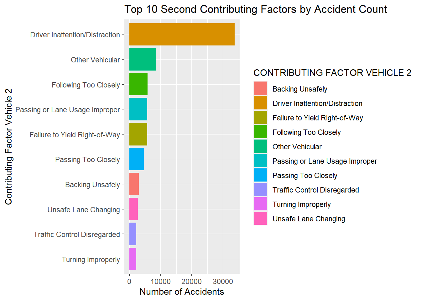 In the above plots, we notice that for both, first and second contributing factors, driver inattention was significantly the most crucial reason that an accident occured for vehicle 1 and 2.
#Vehicle Type EDA
Most of the observations do not have variables CONTRIBUTING FACTOR VEHICLE 5, VEHICLE TYPE CODE 5 etc, and hence, we dropped them, and created a new binary variable which represents if 3 or more vehicles were involved in an accident.
collision_use <- collision_use %>% mutate(VEHICLES_INVOLVED_GTE3 = 1 * !is.na(`CONTRIBUTING FACTOR VEHICLE 3`))
collision_use <- collision_use %>% select(-c(`VEHICLE TYPE CODE 5`,`CONTRIBUTING FACTOR VEHICLE 5`,
`VEHICLE TYPE CODE 4`,`CONTRIBUTING FACTOR VEHICLE 4`,
`VEHICLE TYPE CODE 3`,`CONTRIBUTING FACTOR VEHICLE 3`,
))#Number of Accidents and Number of Deaths for Combinations of Vehicle Types 1 and 2.
collision_by_vehicleTypes <- collision_use %>%
filter(!is.na(`VEHICLE TYPE CODE 1`) & !is.na(`VEHICLE TYPE CODE 2`)) %>%
filter(`VEHICLE TYPE CODE 1` != "UNKNOWN" & `VEHICLE TYPE CODE 2` != "UNKNOWN") %>%
group_by(`VEHICLE TYPE CODE 1`,`VEHICLE TYPE CODE 2`) %>%
summarise(NUMBER_OF_ACCIDENTS=n(),
NUMBER_OF_DEATHS = sum(`NUMBER OF PERSONS KILLED`)) %>%
arrange(desc(NUMBER_OF_ACCIDENTS))## `summarise()` has grouped output by 'VEHICLE TYPE CODE 1'. You can override using the `.groups` argument.#Injuries/Deaths of person type by borough
collision_persontype <- collision_use %>% group_by(BOROUGH) %>% summarise(Ped_Injuries = sum(`NUMBER OF PEDESTRIANS INJURED`), Ped_Deaths = sum(`NUMBER OF PEDESTRIANS KILLED`), Cyclist_Injuries = sum(`NUMBER OF CYCLIST INJURED`), Cyclist_Deaths = sum(`NUMBER OF CYCLIST KILLED`), Motorist_Injuries = sum(`NUMBER OF MOTORIST INJURED`), Motorist_Deaths = sum(`NUMBER OF MOTORIST KILLED`)) %>% mutate(Ped_Fatality_Rate=Ped_Deaths/Ped_Injuries, Cyclist_Fatality_Rate=Cyclist_Deaths/Cyclist_Injuries, Motorist_Fatality_Rate=Motorist_Deaths/Motorist_Injuries)
df1 <- data.frame(collision_persontype$Ped_Fatality_Rate, collision_persontype$Cyclist_Fatality_Rate, collision_persontype$Motorist_Fatality_Rate, collision_persontype$BOROUGH)
df2 <- tidyr::pivot_longer(df1, cols=c('collision_persontype.Ped_Fatality_Rate', 'collision_persontype.Cyclist_Fatality_Rate', 'collision_persontype.Motorist_Fatality_Rate'), names_to='Type',
values_to="Fatality_Rate")
ggplot(df2, aes(x=collision_persontype.BOROUGH, y=Fatality_Rate, fill=Type)) +
geom_bar(stat='identity', position='dodge')+ggtitle('Borough Fatality Rates by Person Type')+ xlab('Borough')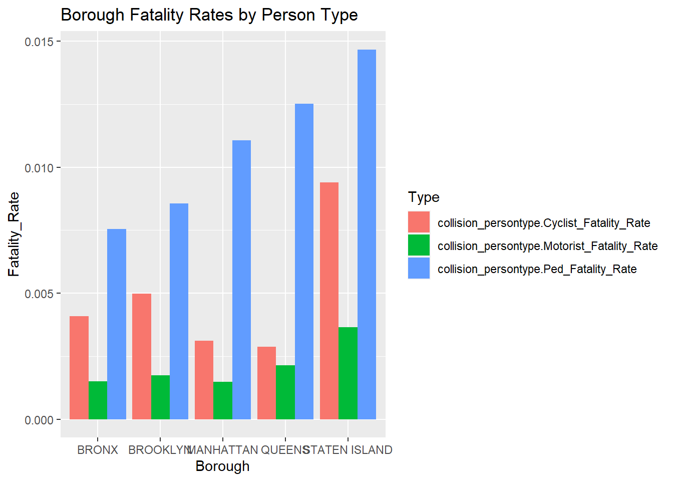 This information is interesting because even though overall accidents were much less in Staten island than in any other borough (Figure 1), here we see that the highest fatality rates in pedestrians and cyclists are in Staten Island. It is also important to note that in every borough, pedestrians face the highest fatality rates consistently, and motorists face the lowest fatality rates consistently. This tells us that pedestrians are at a much higher risk than other types of people.
#Number of Persons Injured by Borough:
collision_use %>% ggplot(aes(x = BOROUGH, y = `NUMBER OF PERSONS INJURED`)) + geom_col()## Warning: Removed 11 rows containing missing values (position_stack).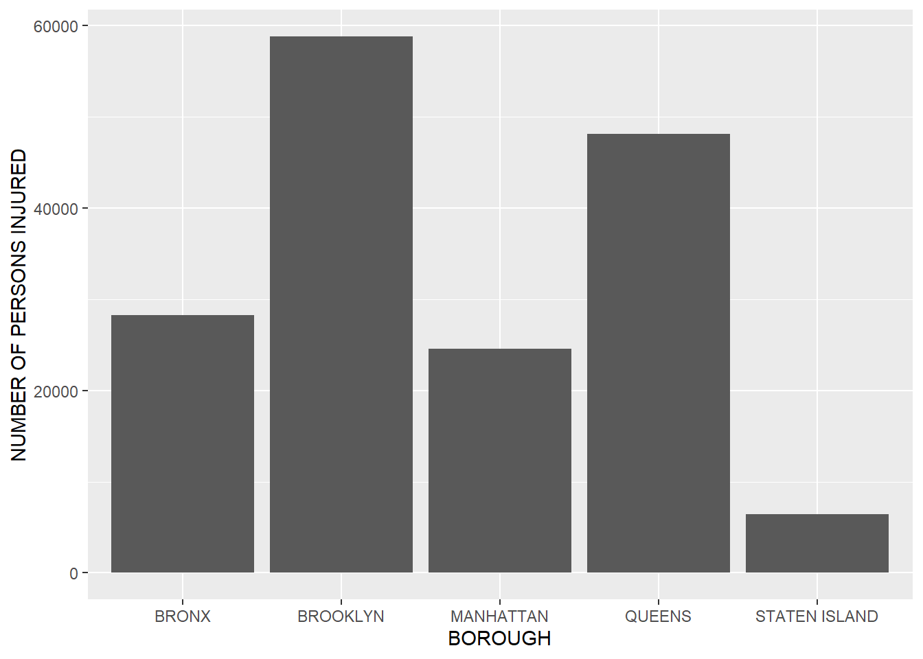 Injuries are directly related to accidents and the highest number of injuries happen where the highest number of accidents occur, i.e. Brooklyn, and vice versa, i.e. Staten Island.
#Further Findings (NYC Collisions Data):
Brooklyn, Queens, and Manhattan have the highest proportions of traffic accidents in New York Ciy. The time of the year when traffic accidents seem to peak is during the summer months of June to October. Interestingly, even though the warmer weather might cause an increase in traffic movement which could potentially lead to an increase traffic collisions, there is a sudden drop in April of traffic accidents. During the day, the most traffic accidents were reported at 4pm and is the lowest at 1am to 2am. Furthermore, in terms of vehicle types, my assumption that sedans were the most prevalent type to be involved in accidents proved true.
In terms of causalities and injuries, my initial assumption that was proven correct where Brooklyn, Manhattan, and Queens have the highest number of people injured and pedestrians killed out of the 5 boroughs.
In terms of the cause of accidents, “unspecified” is the most popular contributing reason for accidents in New York City. Rather than ignoring this, it could either mean that there are certain flaws in the data collecting process that could be improved upon, or there is a wide variety of reasons that the standard choices to do not encompass. There is a possibility that it is a combination of both but I believe this is something that should not be ignored.
Other trends:
-Looking at the volume of accidents by year affirms our initial prediction that 2020 would experience a severe drop in accidents as COVID and quarantine would limit overall driving/traffic in NYC.
-Brooklyn leads all boroughs with the most accidents per year across 5 years, while Staten Island consistently has the least.
-Staten Island also has the lowest population density by far.
-Driver Inattention and Distraction is the largest driver of accidents in NYC. -Approximately 183,000 accidents have cited this as a contributing factor
-Next highest is Failure to Yield Right-of-Way, with approximately 53,000 accidents.
-Staten Island experiences the highest Death to Injury ratio among the boroughs across all types of people. Bronx sees a considerably high death rate for cyclists compared to other boroughs.
-Sedans seem to be involved in the most accidents, with 7 out of the top 10 vehicle code combinations involving sedans.
-Combinations with the most collisions are sedans with other sedans, approximately 95,000 accidents.
#EDA on Weather, Collision Merged Data
library("readxl")
weather <- read_excel(here::here('dataset/WeatherData2016-2020.xlsx'))
weather <- weather %>% rename_with(toupper)
weather <- weather %>% mutate(DAY = ifelse(nchar(DAY) == 1, paste0("0", DAY), DAY))
weather <- weather %>% mutate(MONTH = ifelse(nchar(MONTH) == 1, paste0("0", MONTH), MONTH))
weather <- weather %>% unite("DATE", MONTH, DAY, YEAR, sep = "/")library(tidyverse)
library(dplyr)
library(lubridate)
library(sf)## Linking to GEOS 3.9.1, GDAL 3.2.1, PROJ 7.2.1library(readxl)
library(jtools)
collision <- read_csv(here::here('dataset/NYC Collision Data.csv'))## Rows: 1831755 Columns: 29## -- Column specification --------------------------------------------------------
## Delimiter: ","
## chr (17): CRASH DATE, CRASH TIME, BOROUGH, LOCATION, ON STREET NAME, CROSS S...
## dbl (12): ZIP CODE, LATITUDE, LONGITUDE, NUMBER OF PERSONS INJURED, NUMBER O...##
## i Use `spec()` to retrieve the full column specification for this data.
## i Specify the column types or set `show_col_types = FALSE` to quiet this message.collision_10000 <- collision %>% separate(`CRASH DATE`, c("MONTH", "DAY", "YEAR"), sep = "/") %>%
sample_n(10000) %>%
filter(YEAR != 2012, YEAR != 2015, YEAR != 2013, YEAR != 2014) %>% write_csv("NYC Collision 10000.csv")
collision_use <- collision %>%
filter(!is.na(BOROUGH), !is.na('ZIP CODE'), !is.na(LONGITUDE), !is.na(LATITUDE), !is.na(LOCATION), !is.na(`NUMBER OF PEDESTRIANS KILLED`), !is.na(`NUMBER OF CYCLIST INJURED`)) %>%
select(-(`ON STREET NAME`:`OFF STREET NAME`)) %>%
rename(DATE = `CRASH DATE`, TIME = `CRASH TIME`, ZIPCODE = `ZIP CODE`, LOCATION = `LOCATION`) %>% separate(DATE, c("MONTH", "DAY", "YEAR"), sep = "/") %>%
separate(TIME, c("HOUR", "MINUTE"), sep = ":") %>%
mutate(`CONTRIBUTING FACTOR VEHICLE 1` = str_to_lower(`CONTRIBUTING FACTOR VEHICLE 1`)) %>%
mutate(`CONTRIBUTING FACTOR VEHICLE 2` = str_to_lower(`CONTRIBUTING FACTOR VEHICLE 2`)) %>%
mutate(`CONTRIBUTING FACTOR VEHICLE 3` = str_to_lower(`CONTRIBUTING FACTOR VEHICLE 3`)) %>%
mutate(`CONTRIBUTING FACTOR VEHICLE 4` = str_to_lower(`CONTRIBUTING FACTOR VEHICLE 4`)) %>%
mutate(`CONTRIBUTING FACTOR VEHICLE 5` = str_to_lower(`CONTRIBUTING FACTOR VEHICLE 5`)) %>% filter(!is.na(`CONTRIBUTING FACTOR VEHICLE 1`),!is.na(`CONTRIBUTING FACTOR VEHICLE 2`), !is.na(`CONTRIBUTING FACTOR VEHICLE 3`), !is.na(`CONTRIBUTING FACTOR VEHICLE 4`), !is.na(`CONTRIBUTING FACTOR VEHICLE 5`)) %>%
pivot_longer(`CONTRIBUTING FACTOR VEHICLE 1`:`CONTRIBUTING FACTOR VEHICLE 5`, names_to = "CONTRIBUTING VEHICLE", values_to = "CAUSE") %>% filter(!is.na(CAUSE)) %>%
pivot_longer(`VEHICLE TYPE CODE 1`:`VEHICLE TYPE CODE 5`, names_to = "VEHICLE CODE", values_to = "VEHICLE") %>%
select(-(`CONTRIBUTING VEHICLE`)) %>% select(-(`VEHICLE CODE`)) %>% mutate(VEHICLE = str_to_lower(VEHICLE)) %>%
filter(!is.na("VEHICLE")) %>% sample_n(10000)
collision_10000 <- collision_10000 %>% unite("DATE", MONTH, DAY, YEAR, sep = "/")
collisions_by_day <- collision_10000 %>% group_by(DATE) %>% transmute(`NUMBER OF PERSONS KILLED` = sum(`NUMBER OF PERSONS KILLED`), `NUMBER OF PEDESTRIANS KILLED` = sum(`NUMBER OF PEDESTRIANS KILLED`), `NUMBER OF CYCLIST KILLED` = sum(`NUMBER OF CYCLIST KILLED`), `NUMBER OF MOTORIST KILLED` = sum(`NUMBER OF MOTORIST KILLED`), `NUMBER OF PERSONS INJURED` = sum(`NUMBER OF PERSONS INJURED`), `NUMBER OF PEDESTRIANS INJURED` = sum(`NUMBER OF PEDESTRIANS INJURED`), `NUMBER OF CYCLIST INJURED` = sum(`NUMBER OF CYCLIST INJURED`), `NUMBER OF MOTORIST INJURED` = sum(`NUMBER OF MOTORIST INJURED`))
collisions_by_day <- unique(collisions_by_day)
merged_data <- right_join(collisions_by_day, weather, by = "DATE")
merged_data <- merged_data %>% arrange(DATE)The above code merges the collision data with the weather data. To do this, all accidents that occurred on a given day are grouped into a single row, adding up all the variables present in the data to determine a relationship between weather and traffic collisions.
#Spatial Maps
We will now be using the spatial mapping technique discussed in class to understand the area we are focusing on.
library(tmap)## Registered S3 methods overwritten by 'stars':
## method from
## st_bbox.SpatRaster sf
## st_crs.SpatRaster sflibrary(sf)
collisions_tmap <- collision_10000 %>% filter(!is.na(LONGITUDE), !is.na(LATITUDE), LATITUDE != 0, LONGITUDE != 0, LONGITUDE> -200, !is.na(`ZIP CODE`)) %>% group_by(`ZIP CODE`) %>% mutate(num_collisions=n()) %>% st_as_sf(coords = c("LATITUDE", "LONGITUDE")) %>% st_set_crs(2263)
#print(collisions_tmap, n = 5)
tm_shape(collisions_tmap) + tm_dots(col='num_collisions') 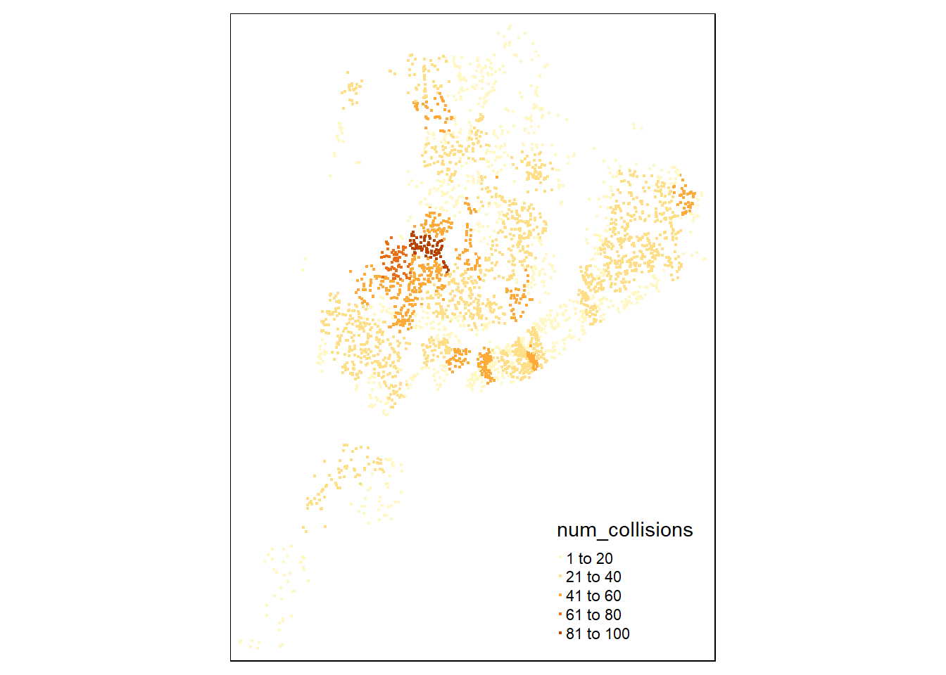 The above map gives us the overall New York area including the five boroughs. This highlights the area we are looking at and we aim to group by boroughs to see which borough has the highest number of accidents.
Relationship between amount of snow, ice pellets, hail, and ice on the ground and the number of people killed in traffic accidents
summ(lm(`NUMBER OF PERSONS KILLED` ~ as.numeric(`SNOW, ICE PELLETS, HAIL, ICE ON GROUND (IN)`), data = merged_data))## Warning in eval(predvars, data, env): NAs introduced by coercion## MODEL INFO:
## Observations: 1665 (162 missing obs. deleted)
## Dependent Variable: NUMBER OF PERSONS KILLED
## Type: OLS linear regression
##
## MODEL FIT:
## F(1,1663) = 0.09, p = 0.77
## R² = 0.00
## Adj. R² = -0.00
##
## Standard errors: OLS
## -------------------------------------------------------------
## Est. S.E. t val. p
## ------------------------------ ------- ------ -------- ------
## (Intercept) 0.00 0.00 2.02 0.04
## as.numeric(`SNOW, ICE -0.00 0.00 -0.29 0.77
## PELLETS, HAIL, ICE ON GROUND
## (IN)`)
## -------------------------------------------------------------Here, there is no correlation between the amount of snow, ice pellets, and hail and the number of people killed in traffic accidents. We see that on average, 0.36 people are killed per day in traffic accidents, with an estimate of -0.02 as the x variable increases by 1, showing that traffic deaths may actually decrease with extreme weather. This is in contrast to what one would expect, as extreme weather creates less safe conditions. However, the likely reason for this is that people both avoid driving and drive slower when the weather is unsafe, reducing traffic volume. This provides another avenue to explore - how the weather relates to the number of cars on the road.
ggplot(merged_data, aes(x = as.numeric(`SNOW, ICE PELLETS, HAIL, ICE ON GROUND (IN)`), y = `NUMBER OF PERSONS KILLED`)) + geom_point() + geom_smooth()## Warning in FUN(X[[i]], ...): NAs introduced by coercion
## Warning in FUN(X[[i]], ...): NAs introduced by coercion

## Warning in FUN(X[[i]], ...): NAs introduced by coercion
## `geom_smooth()` using method = 'gam' and formula 'y ~ s(x, bs = "cs")'## Warning: Removed 162 rows containing non-finite values (stat_smooth).## Warning: Removed 162 rows containing missing values (geom_point).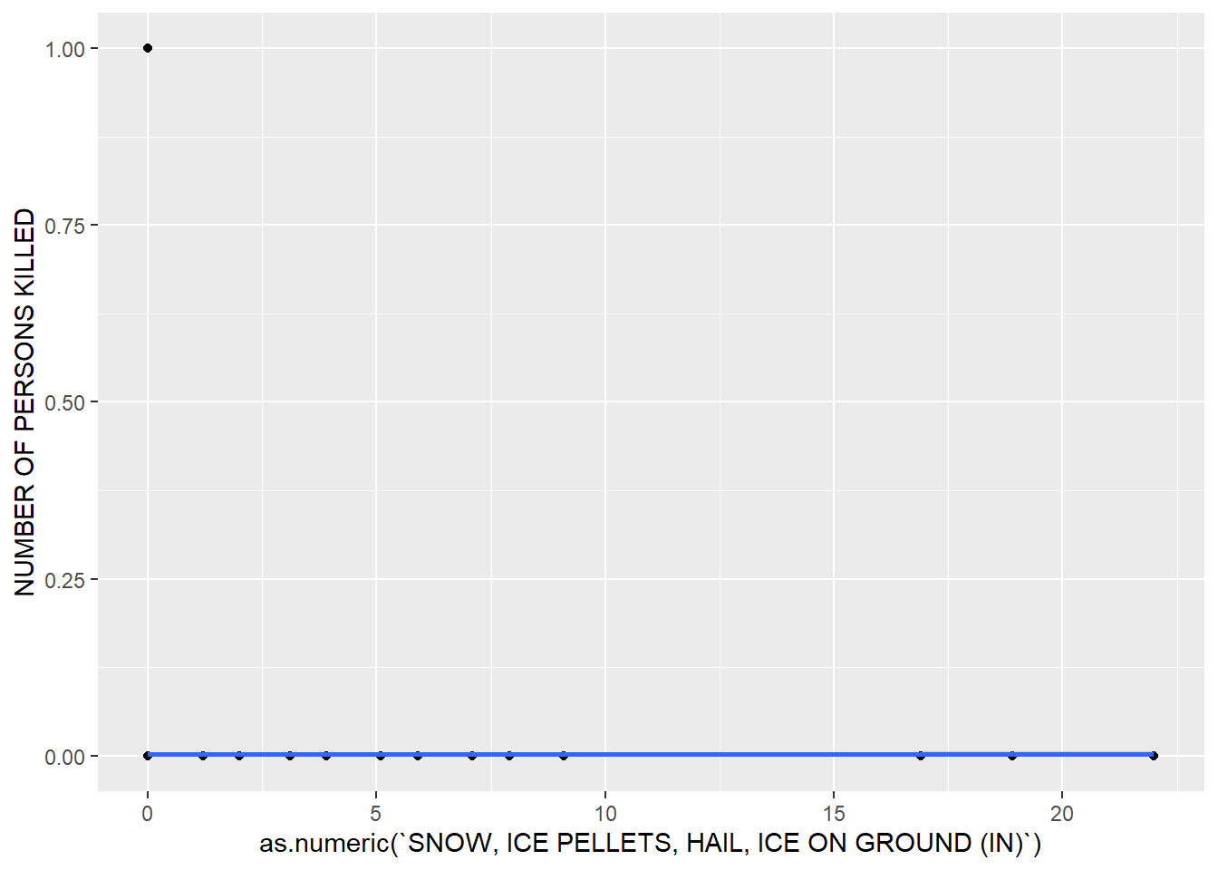
Attempting to visualize the data, it can be seen that days of extreme weather are few and far between over the time interval we chose, so deriving a relationship may not be so easy. If traffic volume is controlled for, the data may change significantly.
Relationship between amount of snow, ice pellets, hail, ice on the ground and the number of people injured in traffic accidents
summ(lm(`NUMBER OF PERSONS INJURED` ~ as.numeric(`SNOW, ICE PELLETS, HAIL, ICE ON GROUND (IN)`), data = merged_data))## Warning in eval(predvars, data, env): NAs introduced by coercion## MODEL INFO:
## Observations: 1665 (162 missing obs. deleted)
## Dependent Variable: NUMBER OF PERSONS INJURED
## Type: OLS linear regression
##
## MODEL FIT:
## F(1,1663) = 4.84, p = 0.03
## R² = 0.00
## Adj. R² = 0.00
##
## Standard errors: OLS
## -------------------------------------------------------------
## Est. S.E. t val. p
## ------------------------------ ------- ------ -------- ------
## (Intercept) 0.97 0.03 28.30 0.00
## as.numeric(`SNOW, ICE -0.07 0.03 -2.20 0.03
## PELLETS, HAIL, ICE ON GROUND
## (IN)`)
## -------------------------------------------------------------ggplot(merged_data, aes(x = as.numeric(`SNOW, ICE PELLETS, HAIL, ICE ON GROUND (IN)`), y = `NUMBER OF PERSONS INJURED`)) + geom_point() + geom_smooth()## Warning in FUN(X[[i]], ...): NAs introduced by coercion## Warning in FUN(X[[i]], ...): NAs introduced by coercion
## Warning in FUN(X[[i]], ...): NAs introduced by coercion## `geom_smooth()` using method = 'gam' and formula 'y ~ s(x, bs = "cs")'## Warning: Removed 162 rows containing non-finite values (stat_smooth).## Warning: Removed 162 rows containing missing values (geom_point).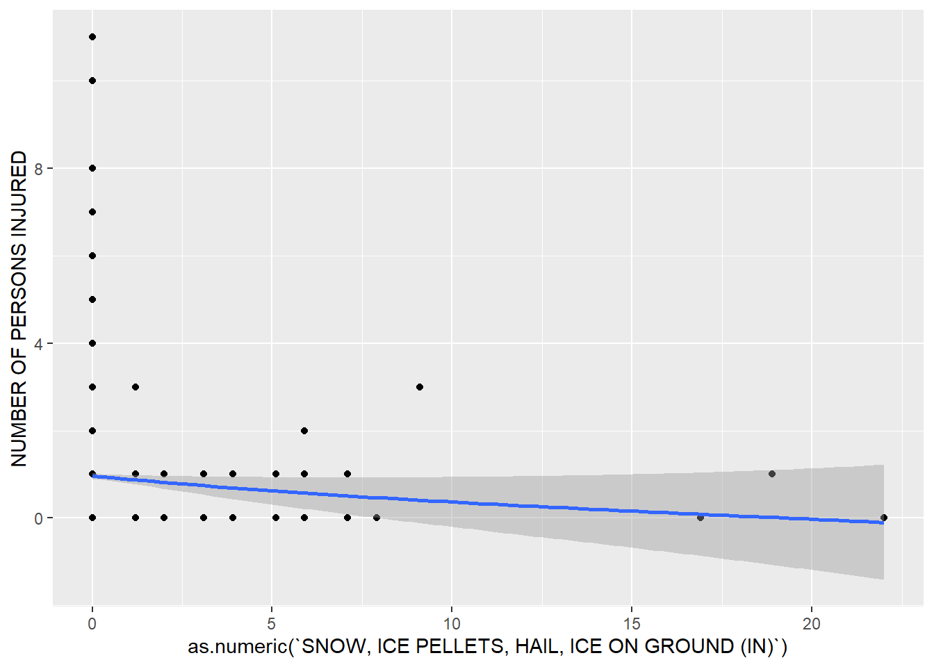
Similar to the number of deaths, in the above plot, there is very little correlation between extreme weather and the number of injuries from traffic-related incidents. As was mentioned before, however, the lack of data points makes it difficult to discern a pattern. The only avenue of exploration with respect to this x variable involves looking at traffic volume.
Relationship between temperature and injuries
summ(lm(`NUMBER OF PERSONS INJURED` ~ `TEMP HIGH`, data = merged_data))## MODEL INFO:
## Observations: 1694 (133 missing obs. deleted)
## Dependent Variable: NUMBER OF PERSONS INJURED
## Type: OLS linear regression
##
## MODEL FIT:
## F(1,1692) = 11.34, p = 0.00
## R² = 0.01
## Adj. R² = 0.01
##
## Standard errors: OLS
## -----------------------------------------------
## Est. S.E. t val. p
## ----------------- ------ ------ -------- ------
## (Intercept) 0.56 0.12 4.53 0.00
## TEMP HIGH 0.01 0.00 3.37 0.00
## -----------------------------------------------ggplot(merged_data) + geom_point(aes(x = `TEMP HIGH`, y = `NUMBER OF PERSONS INJURED`), stat = "identity") + geom_smooth(aes(x = `TEMP HIGH`, y = `NUMBER OF PERSONS INJURED`))## `geom_smooth()` using method = 'gam' and formula 'y ~ s(x, bs = "cs")'## Warning: Removed 133 rows containing non-finite values (stat_smooth).## Warning: Removed 133 rows containing missing values (geom_point).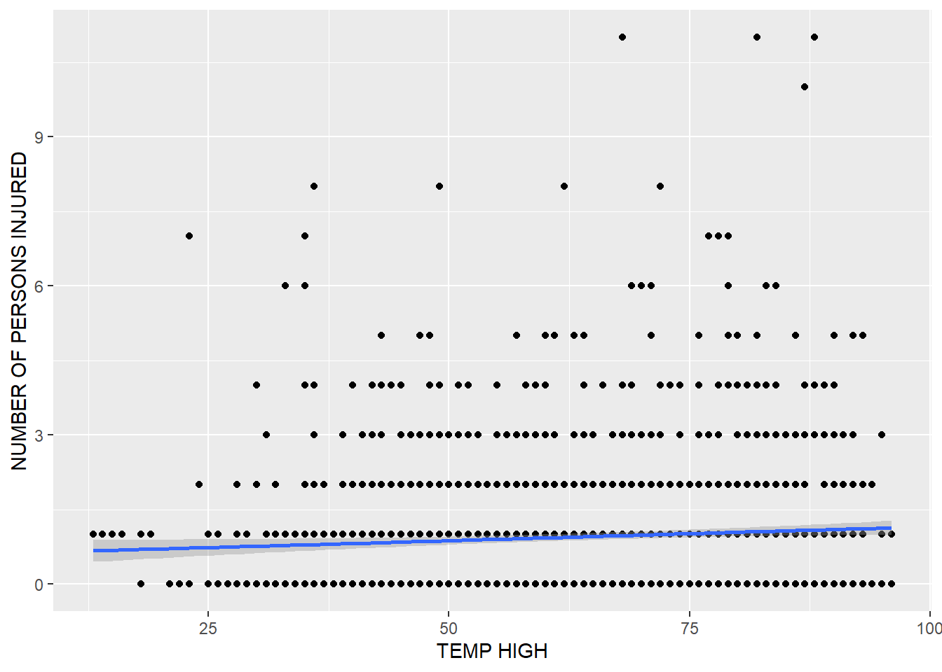
The plot above shows that an increase in temperature by 1 correlates with an increase in number of persons injured by traffic deaths of 0.4. This could be a result of traffic volume, as people travel more in the city (especially to leave to second homes in the summer months).
ggplot(merged_data) + geom_smooth(aes(x = DATE, y = `NUMBER OF PEDESTRIANS INJURED`, group = 1), color = "green") + geom_smooth(aes(x = DATE, y = `NUMBER OF CYCLIST INJURED`, group = 1), color = "blue") + geom_smooth(aes(x = DATE, y = `NUMBER OF MOTORIST INJURED`, group = 1), color = "red")## `geom_smooth()` using method = 'gam' and formula 'y ~ s(x, bs = "cs")'## Warning: Removed 133 rows containing non-finite values (stat_smooth).## `geom_smooth()` using method = 'gam' and formula 'y ~ s(x, bs = "cs")'## Warning: Removed 133 rows containing non-finite values (stat_smooth).## `geom_smooth()` using method = 'gam' and formula 'y ~ s(x, bs = "cs")'## Warning: Removed 133 rows containing non-finite values (stat_smooth).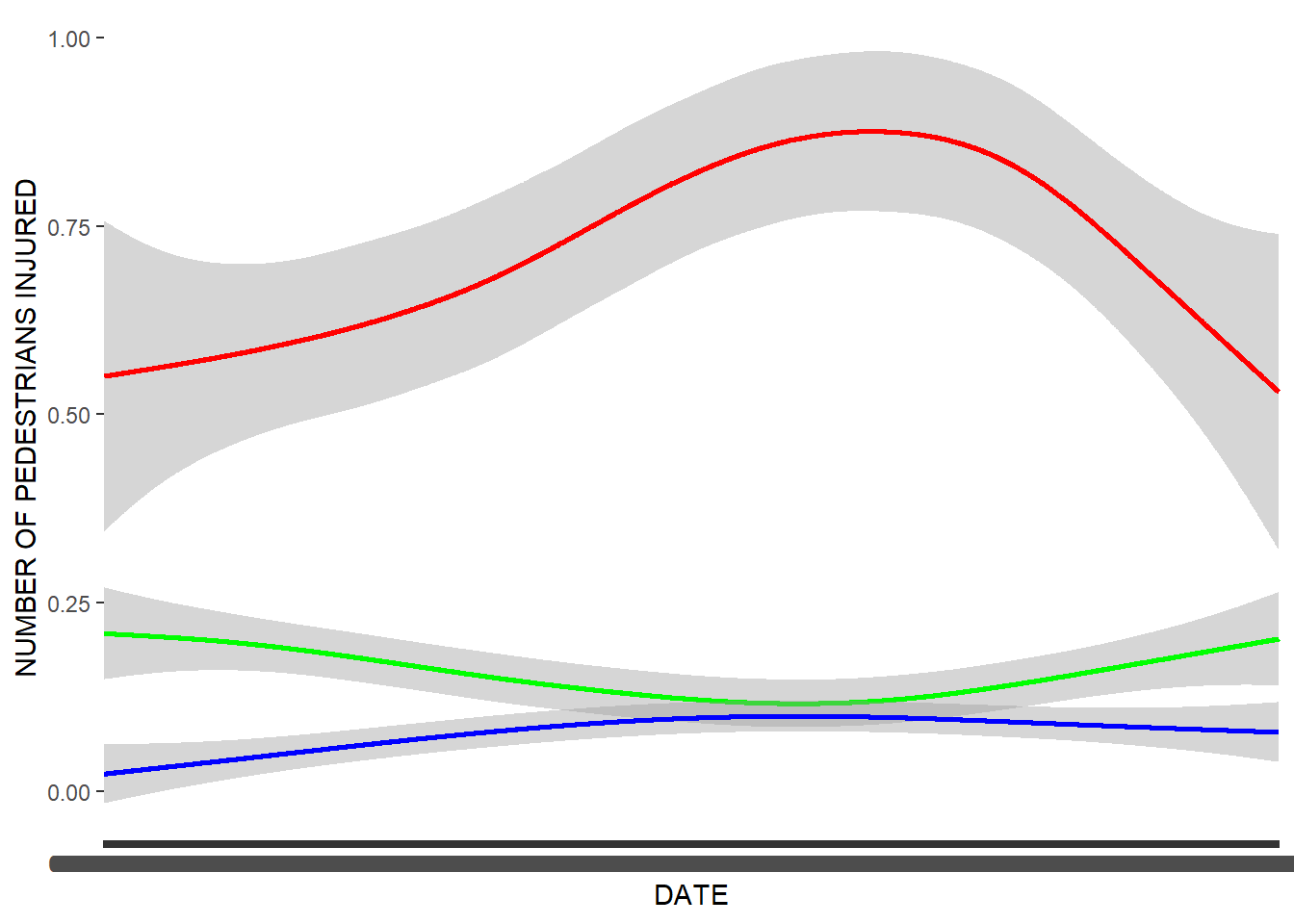
The above graph compares the number of injuries from motorists, pedestrians, and cyclists over the time period we are measuring. Motorists suffer by far the most injuries, followed by pedestrians and the cyclists. This is somewhat surprising, as it is a common belief that cyclists are in an extremely dangerous position. It is worth exploring how the existence of bike paths has affected this number, as well as other policies that affect these different groups.
ggplot(merged_data) + geom_smooth(aes(x = DATE, y = `NUMBER OF PEDESTRIANS KILLED`, group = 1), color = "green") + geom_smooth(aes(x = DATE, y = `NUMBER OF CYCLIST KILLED`, group = 1), color = "blue") + geom_smooth(aes(x = DATE, y = `NUMBER OF MOTORIST KILLED`, group = 1), color = "red")## `geom_smooth()` using method = 'gam' and formula 'y ~ s(x, bs = "cs")'## Warning: Removed 133 rows containing non-finite values (stat_smooth).## `geom_smooth()` using method = 'gam' and formula 'y ~ s(x, bs = "cs")'## Warning: Removed 133 rows containing non-finite values (stat_smooth).## Warning: Computation failed in `stat_smooth()`:
## NA/NaN/Inf in foreign function call (arg 3)## `geom_smooth()` using method = 'gam' and formula 'y ~ s(x, bs = "cs")'## Warning: Removed 133 rows containing non-finite values (stat_smooth).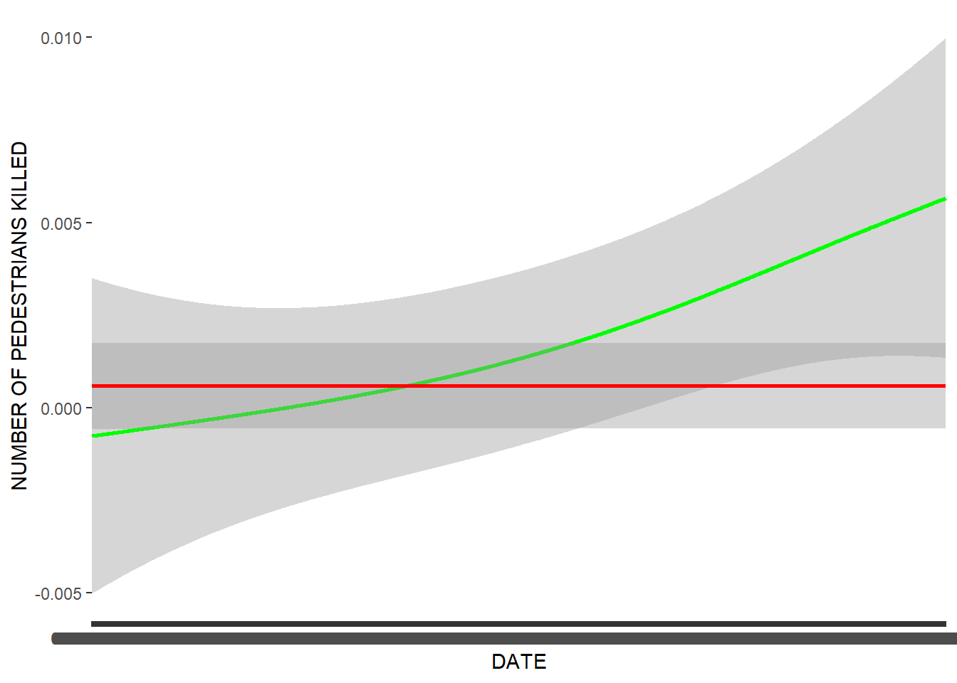
This is the same plot as the previous one but for deaths rather than injuries. Cyclists are still the least likely to be killed. Pedestrians are more likely to be killed than motorists despite being less likely to be injured, suggesting that collisions involving pedestrians are more severe. Further exploration can involve the type of vehicle and the type of collision, further evaluating how these collisions happen to make such situations safer.