#Merging the Weather and Collisions:
library(tidyverse)## -- Attaching packages --------------------------------------- tidyverse 1.3.1 --## v ggplot2 3.3.5 v purrr 0.3.4
## v tibble 3.1.4 v dplyr 1.0.7
## v tidyr 1.1.3 v stringr 1.4.0
## v readr 2.0.1 v forcats 0.5.1## -- Conflicts ------------------------------------------ tidyverse_conflicts() --
## x dplyr::filter() masks stats::filter()
## x dplyr::lag() masks stats::lag()library("readxl")
library(jtools)
weather <- read_excel(here::here('dataset/WeatherData2016-2020.xlsx'))
weather <- weather %>% rename_with(toupper)
weather <- weather %>% mutate(DAY = ifelse(nchar(DAY) == 1, paste0("0", DAY), DAY))
weather <- weather %>% mutate(MONTH = ifelse(nchar(MONTH) == 1, paste0("0", MONTH), MONTH))
weather <- weather %>% unite("DATE", MONTH, DAY, YEAR, sep = "/")
# Merging collision and weather
collisions_10000 <- read_csv(here::here("dataset/NYC Collision 10000.csv"))## Rows: 6118 Columns: 31## -- Column specification --------------------------------------------------------
## Delimiter: ","
## chr (18): MONTH, DAY, CRASH TIME, BOROUGH, LOCATION, ON STREET NAME, CROSS S...
## dbl (13): YEAR, ZIP CODE, LATITUDE, LONGITUDE, NUMBER OF PERSONS INJURED, NU...##
## i Use `spec()` to retrieve the full column specification for this data.
## i Specify the column types or set `show_col_types = FALSE` to quiet this message.collisions_by_day <- collisions_10000 %>% group_by(YEAR, MONTH, DAY) %>% transmute(`NUMBER OF PERSONS KILLED` = sum(`NUMBER OF PERSONS KILLED`), `NUMBER OF PEDESTRIANS KILLED` = sum(`NUMBER OF PEDESTRIANS KILLED`), `NUMBER OF CYCLIST KILLED` = sum(`NUMBER OF CYCLIST KILLED`), `NUMBER OF MOTORIST KILLED` = sum(`NUMBER OF MOTORIST KILLED`), `NUMBER OF PERSONS INJURED` = sum(`NUMBER OF PERSONS INJURED`), `NUMBER OF PEDESTRIANS INJURED` = sum(`NUMBER OF PEDESTRIANS INJURED`), `NUMBER OF CYCLIST INJURED` = sum(`NUMBER OF CYCLIST INJURED`), `NUMBER OF MOTORIST INJURED` = sum(`NUMBER OF MOTORIST INJURED`))
collisions_by_day <- unique(collisions_by_day) %>% unite("DATE", MONTH, DAY, YEAR, sep = "/")
merged_data <- right_join(collisions_by_day, weather, by = c('DATE'))
merged_data <- merged_data %>% arrange(DATE) summ(lm(`NUMBER OF PERSONS INJURED` ~ `TEMP LOW`, data = merged_data))## MODEL INFO:
## Observations: 1703 (124 missing obs. deleted)
## Dependent Variable: NUMBER OF PERSONS INJURED
## Type: OLS linear regression
##
## MODEL FIT:
## F(1,1701) = 15.13, p = 0.00
## R² = 0.01
## Adj. R² = 0.01
##
## Standard errors: OLS
## -----------------------------------------------
## Est. S.E. t val. p
## ----------------- ------ ------ -------- ------
## (Intercept) 0.57 0.10 5.52 0.00
## TEMP LOW 0.01 0.00 3.89 0.00
## -----------------------------------------------ggplot(merged_data) + geom_point(aes(x = `TEMP LOW`, y = `NUMBER OF PERSONS INJURED`), stat = "identity") + geom_smooth(aes(x = `TEMP LOW`, y = `NUMBER OF PERSONS INJURED`))## `geom_smooth()` using method = 'gam' and formula 'y ~ s(x, bs = "cs")'## Warning: Removed 124 rows containing non-finite values (stat_smooth).## Warning: Removed 124 rows containing missing values (geom_point).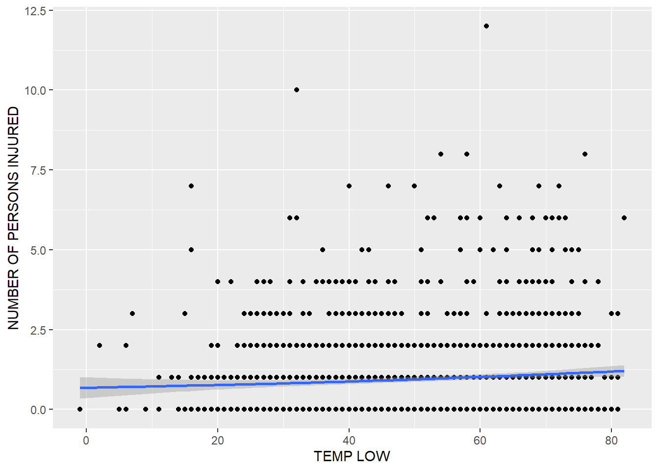 We noticed in our EDA in a previous blog post that there is a slight correlation between the high temperature on a given day and the number of injuries. This was reflected by a correlation coefficient of 0.08 and a beta of 0.4, suggesting that as temperature increases by 1, the number of injuries increases by 0.4. I test here to see if the relationship holds for the low temperature as well, which is it does. The correlation coefficient is equivalent at 0.08, and the beta is slightly higher at 0.44.
merged_data <- merged_data %>% separate(DATE, c("MONTH", "DAY", "YEAR"), sep = "/")

# Here, the date is being separated in order to work directly with the "MONTHS" variable.

merged_data <- merged_data %>% mutate(SEASON = case_when(MONTH %in% c("09", "10", "11") ~ "Fall", MONTH %in% c("12", "01", "02")  ~ "Winter", MONTH %in% c("03", "04", "05")  ~ "Spring", TRUE ~ "Summer"))
Here, the season is being coded into each data point. The logical conclusion from the relationship between temperature and injuries is a change in traffic conditions in New York between seasons. For example, in the summer, many people leave New York City to go to second homes, which increases traffic, especially on the weekends, but reduces travel within the city itself. This provides a major area of discussion by which to build our model.
summ(lm(`NUMBER OF PERSONS INJURED` ~ `MONTH`, data = merged_data))## MODEL INFO:
## Observations: 1703 (124 missing obs. deleted)
## Dependent Variable: NUMBER OF PERSONS INJURED
## Type: OLS linear regression
##
## MODEL FIT:
## F(11,1691) = 1.66, p = 0.08
## R² = 0.01
## Adj. R² = 0.00
##
## Standard errors: OLS
## ------------------------------------------------
## Est. S.E. t val. p
## ----------------- ------- ------ -------- ------
## (Intercept) 0.91 0.11 8.09 0.00
## MONTH02 -0.09 0.16 -0.55 0.59
## MONTH03 -0.23 0.16 -1.42 0.16
## MONTH04 0.06 0.16 0.36 0.72
## MONTH05 0.10 0.16 0.59 0.55
## MONTH06 -0.06 0.16 -0.38 0.71
## MONTH07 0.02 0.16 0.14 0.89
## MONTH08 0.08 0.16 0.52 0.61
## MONTH09 0.35 0.16 2.19 0.03
## MONTH10 0.18 0.16 1.12 0.26
## MONTH11 0.14 0.16 0.86 0.39
## MONTH12 -0.03 0.16 -0.18 0.86
## ------------------------------------------------ggplot(merged_data) + geom_bar(aes(x = `MONTH`, y = `NUMBER OF PERSONS INJURED`, fill = SEASON), stat = "identity")## Warning: Removed 124 rows containing missing values (position_stack).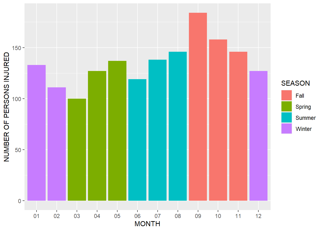 The plot and linear regression below show a clear relationship between the month and the number of people injured from traffic accidents. The numbers are the highest in the summer, followed by the fall and then winter and spring. Evaluating further the workings of New York City and how the time of year affects traffic collisions will be a major point of focus in our model.
summ(lm(`NUMBER OF PERSONS INJURED` ~ `SEASON`, data = merged_data))## MODEL INFO:
## Observations: 1703 (124 missing obs. deleted)
## Dependent Variable: NUMBER OF PERSONS INJURED
## Type: OLS linear regression
##
## MODEL FIT:
## F(3,1699) = 3.48, p = 0.02
## R² = 0.01
## Adj. R² = 0.00
##
## Standard errors: OLS
## -------------------------------------------------
## Est. S.E. t val. p
## ------------------ ------- ------ -------- ------
## (Intercept) 1.13 0.07 17.29 0.00
## SEASONSpring -0.25 0.09 -2.70 0.01
## SEASONSummer -0.21 0.09 -2.25 0.02
## SEASONWinter -0.26 0.09 -2.81 0.00
## -------------------------------------------------ggplot(merged_data) + geom_bar(aes(x = `SEASON`, y = `NUMBER OF PERSONS INJURED`, fill = SEASON), stat = "identity")## Warning: Removed 124 rows containing missing values (position_stack).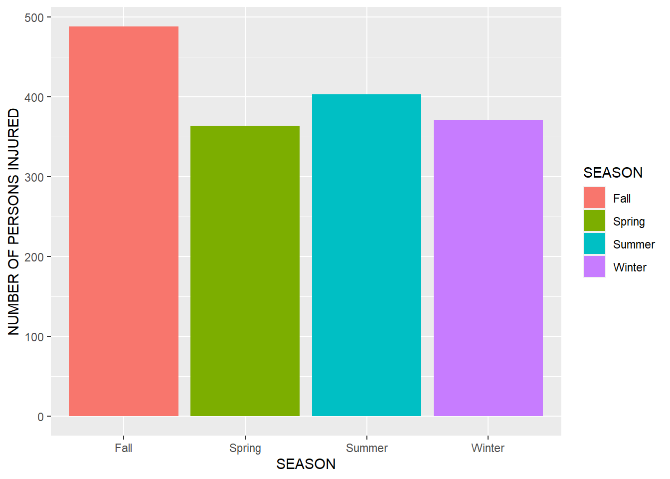 The plot below is similar to the previous one but with the seasons grouped together for a simpler visualization.
Stepping away from the weather data, we aim to dig deeper into the original dataset by looking at any drastic changes in the traffic volume over our 5 period horizon. In order to do so, we looked into recent traffic laws and guidelines related to motorists, cyclists, and pedestrians to see if there is any difference after the laws have been implemented. For example, in recent years, there has been much discussion about lowering the legal blood alcohol limit from 0.08 to 0.05 under a proposed new bill. New York state lawmakers and bill sponsor state Sen. John Liu is looking to lower this limit in future legislation sessions as a top priority. The National Transportation Safety Board in 2012 actually advised states to lower the limit to 0.05 but Utah is the only state to have done so. 114 nations have lower limits than the US and lawmakers predict that lowering the limit could potentially save 25 lives per year in New York.
In 2019, the proposal was met with both support and criticism where critics were saying that for a tragedy to be fatal the average BAC is around 0.16 and 0.17. Our research could potentially add to showing the probability of a death occurring if alcohol was or was not a contributing factor in the accident.
Using a logistic regression model with a independent variable that represents whether or not alcohol was a Contributing Factor in the Collision (0: No Alcohol, 1: Alcohol), and a binary dependent variable (whether or not collision results in a death; 0: No Death, 1: Death), we can determine how much more likely is that a death will occur if alcohol is involved as a Contributing Factor. This paradigm for logistic regression analysis can also be done on some of the other notable Contributing Factors, to determine how each contributing factor influences the probability of death in a collision. For example, we could explore how much more likely death would be if one of the Contributing Factors in the collision was “Driver Inattention/Distraction.”
Additionally, we believe the “HOUR” variable could be extremely interesting as there are definitely peak hours of traffic such as when offices open and close, lunch hours, etc. We predict that most accidents occur during these peak hours. We will be running a fit model to further discuss our findings on this prediction.
To throw more light on this topic, we will be focusing on motorists, cyclists, and pedestrians separately as we discuss the variable “HOUR” since perhaps, during lunch hour, for example, pedestrian traffic volume will be significantly higher than motorist traffic volume.
Lastly, in the last five years, the Department of Transportation has expanded and enhanced the on-street bike network by more than 330 miles, including more than 82 protected lane miles, with 20 miles installed in 2018. It has installed over 66 lane miles of bike facilities, including 55 lane miles of dedicated cycling space in 2018. Through a fit model between cyclists, number of injuries and year, we will be examining the number of accidents for cyclists, before and after these installations to observe differences, if any.
Updated Blog Post 5 with Data Loading, Cleaning and Merging:
In our previous blog post, we ran a few correlations on the merged data set including the original collision dataset and the weather dataset. Specifically, we observed a very low correlation of only 0.4 between temperatures and injuries and surprisingly, no correlation between the amount of snow, ice pellets and hail, and the number of people killed in traffic accidents. A potential idea is to explore if weather relates to the number of cars on the roads as the lack of correlation might be a result of people avoiding the roads during bad weather.
Even though temperatures and number of injuries do not seem to be too interesting to model, we decided to categorize the weather into seasons and then run an initial fit model to see if anything interesting shows up. For example, we predict that during holiday seasons, pedestrian and cyclist traffic volume might not be as much as during regular working days since people usually travel by air or trains, and hence, we might see a significant drop in the number of injuries or death among those.